Spark optimization（Spark 优化）

This page explains strategies and best practices for optimizing Spark pipelines. It covers both foundational and advanced concepts for building efficient pipelines on the Palantir platform.

Basic optimization

Three core principles guide basic Spark optimization:

Concept	Description
Reduce the data volume	Filter out unneeded rows early and drop unused columns. Keep filter expressions simple and specific.
Repartition	Balance the number of partitions against the number of executors by adjusting how files or partitions split.
Clean the data	Standardize values before processing. For example, normalize Spark and spark to a single casing. Spark treats differently cased strings as distinct values.

Reduce the data volume

A straightforward way to improve Spark performance is to remove unneeded data as early as possible. Two techniques help:

1. Reorder operations so that filters, ordering steps, and inner joins execute in earlier stages.
2. Drop columns that downstream logic does not require.

:::callout{theme="warning"} Spark executes operations exactly as written. To avoid unexpected behavior, ensure your data is cleaned and standardized and that filters target precise values. :::

Splitting or sorting on Parquet metadata (which Spark applies automatically) only benefits downstream performance when the input data is already clean and filtered.

:::callout{theme="neutral"} What are some examples of inefficient filters? Using a user-defined function (UDF) in DataFrames when an equivalent DataFrame API method already exists. :::

Why reducing data volume matters

Filtering early and dropping unused columns reduces the network I/O and disk I/O that each task performs, which improves overall job runtime.

Operation order matters. If you defer dropping unneeded data until a late stage, Spark processes that data through every preceding stage. Dropping it first eliminates that overhead. Note that the cost-based optimizer handles this reordering automatically when enabled.

For example, if D is a dataset that you inner join to datasets SMALL and BIG, this query:

SELECT * FROM D JOIN SMALL ON SMALL.key = D.key JOIN BIG ON BIG.key2 = D.key2

performs better than:

SELECT * FROM D JOIN BIG ON BIG.key2 = D.key2 JOIN SMALL ON SMALL.key = D.key

Restricting the column set on D, BIG, and SMALL improves performance further. Note that when Spark knows the sizes of SMALL and BIG, it attempts to keep the larger dataset in place automatically.

Blind optimization

Blind optimization aims to improve Spark performance regardless of the specific operation. The general goal is to match the number of input splits to the number of executors. The correct executor count depends on your available resources and the workload.

Use the following approximations for the number of splits:

Structure	Splits
Input files are split-compatible, not partitioned	number of splits = number of executors = (file size / HDFS block size)
Input files are split-compatible, partitioned	number of splits = number of executors = number of partitions
Input files are not split-compatible	number of splits = number of executors = number of input files

In the last case, when input files are not split-compatible, Spark must fetch all blocks that compose a file before processing it. The read overhead therefore exceeds that of reading a single file under BLOCK_SIZE.

At worst, blind optimization can assign more data per node than that node can handle, which aborts the job. In that case, increase the number of tasks. Keep in mind that joins can produce output larger than the sum of the input datasets (when join keys match multiple rows). Matching input splits to executors can also cause problems when you aggregate and join, because the operation can produce groups that exceed available memory.

When you know the operation that will run, you can apply operation-aware optimizations. These let you control the number of partitions (or input splits) to reduce shuffling during computation. The two operation-aware optimizations are: 1) bucketing and 2) partitioning.

Clean data

Spark does not infer intent from string content. Internally, Spark converts each unique string to a numeric identifier, and any difference in the string—including casing—produces a separate identifier. For example, Spark assigns 'filter' one integer and 'Filter' a different integer, which prevents it from recognizing that both represent the same value. To avoid this problem, make string filters case-sensitive (for example, filter for both 'filter' and 'Filter') and clean data before processing (for example, normalize all variants to a consistent case without extra characters).

Advanced optimization

The basic methods above are the minimum steps you should take for every pipeline. When they are not sufficient, the techniques in this section can help. Four goals guide advanced optimization:

1. Distribute data across multiple executors (partition) either evenly or by the correct key.
2. Keep task inputs small enough to fit in executor memory.
3. Reduce network I/O and disk I/O, which means limiting file count.
4. Reduce the number of tasks, because each task adds scheduling overhead.

Seven data-formatting methods address these goals. Which methods apply depends on your workload and priorities.

Method	Alternative terms	Description	Affected step	When to use	When not to use
Basic partitioning: Coalesce	Coalesce, changing partition count, DataFrame partitioning, data formatting, repartitioning	Decrease the number of partitions between tasks, which reduces the total task count.	Step 2 (RDD to Executor)	After a task completes and you want fewer output partitions.	When the task does not significantly change the data volume.
Basic partitioning: Repartition by value	Repartition, DataFrame partitioning, data formatting, partitioning by key	After computation, redistribute rows into new partitions based on a specific column value (for example, name or ID).	Step 2 (RDD to Executor)	When the partition column has a small number of distinct values (low cardinality).	When the partition column has many distinct values (approximately greater than 1,000).
Hash partitioning	Bucketing (and sorting)	Create sorted partitions in the RDD based on metadata. Output files use bucket identifiers (output.bucket1.parquet) rather than value names.	Step 3 (Executor to Output File)	When downstream computations match row keys (aggregates, joins) or when pre-sorting benefits multiple use cases.	When there is no clear downstream benefit. Use bucketing only when you have a specific performance goal.
Hive partitioning	Dynamic partitioning, partitioning	After computation, split results into output files organized by a partition key, stored in subdirectories named for each key value.	Step 3 (Executor to Output File)	Large datasets with low-cardinality columns where filter pruning provides significant benefit.	When the result would be too many small files.
Joins and aggregates	—	Materialize a joined or aggregated dataset so that downstream transforms and services reuse it instead of recomputing the join.	N/A	When multiple downstream consumers repeatedly join these datasets (for example, in Contour).	When the unfiltered, joined dataset is too large, or when the join runs infrequently and the additional pipeline step harms overall performance.
Split the transforms	—	Break a single transform into multiple transforms to isolate intermediate steps.	N/A	When other techniques have failed, or when separate steps improve ease of debugging and manageability, or when you need to persist intermediate state.	When the techniques above already provide adequate performance.
Increase resources	—	Allocate additional Foundry resources to your transform. Increasing resources for one transform adds load to the cluster and can reduce performance for other services.	All steps	As a last resort, only when no other option produces acceptable performance and you have an urgent need.	In all other cases.

Basic partitioning: Coalesce (changing partition count)

Coalesce accepts a target partition count and processes multiple input partitions sequentially within a single task.

Advantage: Coalesce works well when you have a large volume of roughly well-distributed data (for example, terabytes). It avoids the cost of redistributing data across the cluster.

Disadvantage: Coalesce does not redistribute data, so output tasks can remain unevenly sized.

```java tab="Java" df.coalesce(N);

```python tab="Python"
df.coalesce(N)

SQL does not support this operation.

Basic partitioning: Repartition by value

Repartitioning by value resembles coalesce, but it hashes each row and redistributes data evenly across the cluster.

Advantage: Produces evenly distributed data, which results in more predictable file sizes.

Disadvantage: Spark writes the dataset to scratch space and transfers it over the network. This cost grows with dataset size, so avoid repartitioning large datasets when the redistribution overhead outweighs the benefit.

```java tab="Java" df.repartition(N);

```python tab="Python"
df.repartition(N)

SQL does not support this operation.

In SparkSQL, you can also repartition by a given set of columns, which hashes those columns instead of the entire row. This technique is discussed in later sections. Note that column-based repartitioning does not inform the Spark query planner when it reads the output files.

```java tab="Java" df.repartition(N, "column1");

```python tab="Python"
df.repartition(N, "column1")

```sql tab="SQL" DISTRIBUTE BY column1

### Hash partitioning (bucketing and sorting)

The basic partitioning methods above are the first techniques to try for improving pipeline performance. However, because Palantir uses SparkSQL throughout, you can extend optimization further by writing datasets in a format that benefits the SparkSQL query planner. SparkSQL lets you write metadata that describes how a dataset is partitioned and the sort order within each partition, which it can then use to skip expensive operations downstream. Two methods provide this: 1) bucketing (and sorting) and 2) Hive partitioning.

**Bucketing** groups rows by key into output files, which accelerates computations that match keys across rows (joins, group-by operations). When you have multiple inputs, bucket all of them for the best results. Bucketing resembles partitioning but places multiple values per partition rather than a single value. Choosing the right bucket count requires balancing several constraints—the goal is to create files that:

* Fit on each node (to use available space) without exceeding node capacity (to avoid crashes)
* Are no smaller than the HDFS block size
* Follow the one-to-one principle of partitions to tasks to executors (unless doing so contradicts the previous constraints)

:::callout{theme="neutral"}
Bucketing and sorting benefit large datasets, but you must understand or control your data distribution before applying them. Bucketing alone helps, but combining bucketing with sorting yields the best results.
:::

The general recommendation is to target output files (buckets) of 128–512 MB. If you perform numerous large joins, you may need to adjust these targets.

Even when an input partition is 128 MB, computation can expand the data. A 128 MB input partition can produce a 512 MB output file.

#### Bucketing with SparkSQL

:::callout{theme="neutral"}
SQL statements that use `CREATE TABLE`—including the bucketing and sorting operations described below—cannot run in Code Workbook. To bucket with SQL, use a Code Repository with the syntax below.
:::

```sql
CREATE TABLE `/path/to/output` USING parquet
CLUSTERED BY (a)
SORTED BY (a)
INTO 200 BUCKETS AS (
SELECT a, b, c
FROM `/path/to/dataset`
CLUSTER BY a
)

The query above uses two separate SQL commands that serve different purposes:

• CLUSTERED BY (and SORTED BY) modify the CREATE TABLE statement to specify the physical layout of the table. These keywords control the actual bucketing into separate files.
• CLUSTER BY is a data operation that triggers a shuffle so that tasks within the cluster group data by the specified key. This step is generally necessary because each Spark task and executor operates independently. Without CLUSTER BY, each task buckets only the data in its own executor memory.

Example: why CLUSTER BY matters

Consider a case with 200 final tasks, bucketing by a key that has 200 possible values. Without CLUSTER BY, those 200 values spread evenly across all 200 tasks. Each task creates one file per key value it encounters, producing 200 × 200 = 40,000 files. This file count causes the read overhead for the next pipeline step to increase sharply.

You can omit CLUSTER BY if you know that each task already owns data with a nearly one-to-one relationship to the bucketing key (for example, after a GROUP BY). Omitting it saves a shuffle, but monitor the number of output files carefully.

Note: The SQL interface to Spark does not always produce the expected result (that is, one file per bucket). If you cannot adjust the SQL to achieve the desired output, use Python instead.

numPartitions controls the number of output files. The shuffle parameter forces a rebalance of data across files. If your input is already well-balanced, set shuffle to false to improve performance. If your input is unbalanced—or if the transformation creates imbalance (for example, a filter that only matches rows in some input files)—set shuffle to true.

In Python, two methods correspond to the shuffle/no-shuffle options. The no-shuffle equivalent (shuffle: false):

df.coalesce(N)

The shuffle equivalent (shuffle: true):

df.repartition(N)

Example: Bucketing a claims dataset

You have a claims dataset, and most of your analysis involves window functions over a given patient_id, joins on patient_id to bring in reference data, or aggregations.

By default, this query:

SELECT claims.patient_id, age FROM claims LEFT JOIN patients on claims.patient_id = patients.patient_id

Produces this physical plan:

== Physical Plan ==*Project [patient_id#50, age#52]+- SortMergeJoin [patient_id#50], [patient_id#51], LeftOuter:- *Sort [patient_id#50 ASC NULLS FIRST], false, 0:  +- Exchange hashpartitioning(patient_id#50, 200):     +- *FileScan parquet default.claims[patient_id#50] Batched: true, Format: Parquet, Location: InMemoryFileIndex[file:/Volumes/git/spark/spark-warehouse/claims], PartitionFilters: [], PushedFilters: [], ReadSchema: struct<patient_id:string>+- *Sort [patient_id#51 ASC NULLS FIRST], false, 0+- Exchange hashpartitioning(patient_id#51, 200)+- *FileScan parquet default.patients[patient_id#51,age#52] Batched: true, Format: Parquet, Location: InMemoryFileIndex[file:/Volumes/git/spark/spark-warehouse/patients], PartitionFilters: [], PushedFilters: [], ReadSchema: struct<patient_id:string,age:int>

The Exchange after each FileScan indicates that Spark shuffles the table by patient_id into 200 partitions, sorts each partition by patient_id, and then performs the SortMergeJoin. With 100 GB of claims and 1 GB of patients, this produces a resource-intensive job because Spark must redistribute all of that data across the cluster.

You can trade write-time cost for faster read-time by rewriting both claims and patients with bucketing metadata:

```java tab="Java" DatasetFormatSettings format = DatasetFormatSettings.builder() .numBuckets(200) .addBucketColumns("patient_id") .addSortColumns("patient_id") .build();

output.getDataFrameWriter(df) .setFormatSettings(format) .write();

```python tab="Python (Code Repository)"
output.write_dataframe(df,bucket_cols=["patient_id"],bucket_count=200,sort_by=["patient_id"])

```python tab="Python (Code Workbook)" from vector.api import DataFrameReturn

def my_vector_node(my_input): return DataFrameReturn(my_input, bucket_cols=["patient_id"], bucket_count=200, sort_by=["patient_id"])

```sql tab="SQL"
CREATE TABLE `claims` USING parquet
CLUSTERED BY (patient_id)
SORTED BY (patient_id)
INTO 200 BUCKETS AS
SELECT ...

The same query now produces this physical plan:

== Physical Plan ==*Project [patient_id#72, age#73]+- SortMergeJoin [patient_id#72], [patient_id#75], LeftOuter:- *FileScan parquet default.claims[patient_id#72,age#73] Batched: true, Format: Parquet, Location: InMemoryFileIndex[file:/Volumes/git/spark/spark-warehouse/claims], PartitionFilters: [], PushedFilters: [], ReadSchema: struct<patient_id:string,age:int>+- *FileScan parquet default.patients[patient_id#75] Batched: true, Format: Parquet, Location: InMemoryFileIndex[file:/Volumes/git/spark/spark-warehouse/patients], PartitionFilters: [], PushedFilters: [], ReadSchema: struct<patient_id:string>

Because Foundry stores metadata about bucketing and sorting, Spark starts the join immediately after fetching data from HDFS or S3. This eliminates the shuffle and sort stages, which reduces job runtime. No local disk writes occur and no additional network traffic beyond the initial fetch is required.

How bucketing affects the write side

Bucketing and sorting do not change the transformation itself—they only control how the final tasks of the job write output. Using the claims example: instead of writing output data sequentially to a single file, Spark creates a temporary column, bucket, defined as hash(patient_id) % 200, and then sorts within the partition by (bucket, patient_id). If your input data looks like this:

A
C
A
A
B
C

Spark formats it as follows (assuming A and B hash to 0 and C hashes to 1):

0 A
0 A
0 A
0 B
1 C
1 C

Spark then scans through the partition and writes a separate file for each bucket value—two files in this case.

If you run repartition(200, "patient_id") immediately before writing, each task produces a single file because the bucket value is constant within each task. However, with evenly distributed data, the worst case is that each task writes 200 individual files. With 200 output tasks, that produces 40,000 output files, which degrades both write and read performance. A high file count also affects Foundry Catalog and Cassandra performance, so limit the number of output files as much as possible.

Hive partitioning

"Partitioning" is an overloaded term in Spark. Documentation typically distinguishes this variant with the labels "Hive-style," "directory," or "dynamic" partitioning.

Hive partitioning occurs in step three. Apache Hive is a system for storing, querying, and analyzing large datasets in a distributed computing environment.

Hive partitioning writes data in the same way as bucketing, but adds a partition column to the output sort. Spark uses this column to organize data into subdirectories—it produces at least one output file for each unique value in the partition column. Because of this, use Hive partitioning for low-cardinality columns (columns with many repeated values) where filter pruning provides measurable benefit.

:::callout{theme="neutral"} As with bucketing, Hive partitioning can produce too many small files if you are not careful. :::

:::callout{theme="neutral"} Both bucketing and Hive partitioning break the one-to-one principle. They either output a different number of files than tasks or rearrange which data each task writes, so the result is not necessarily one output file per task. :::

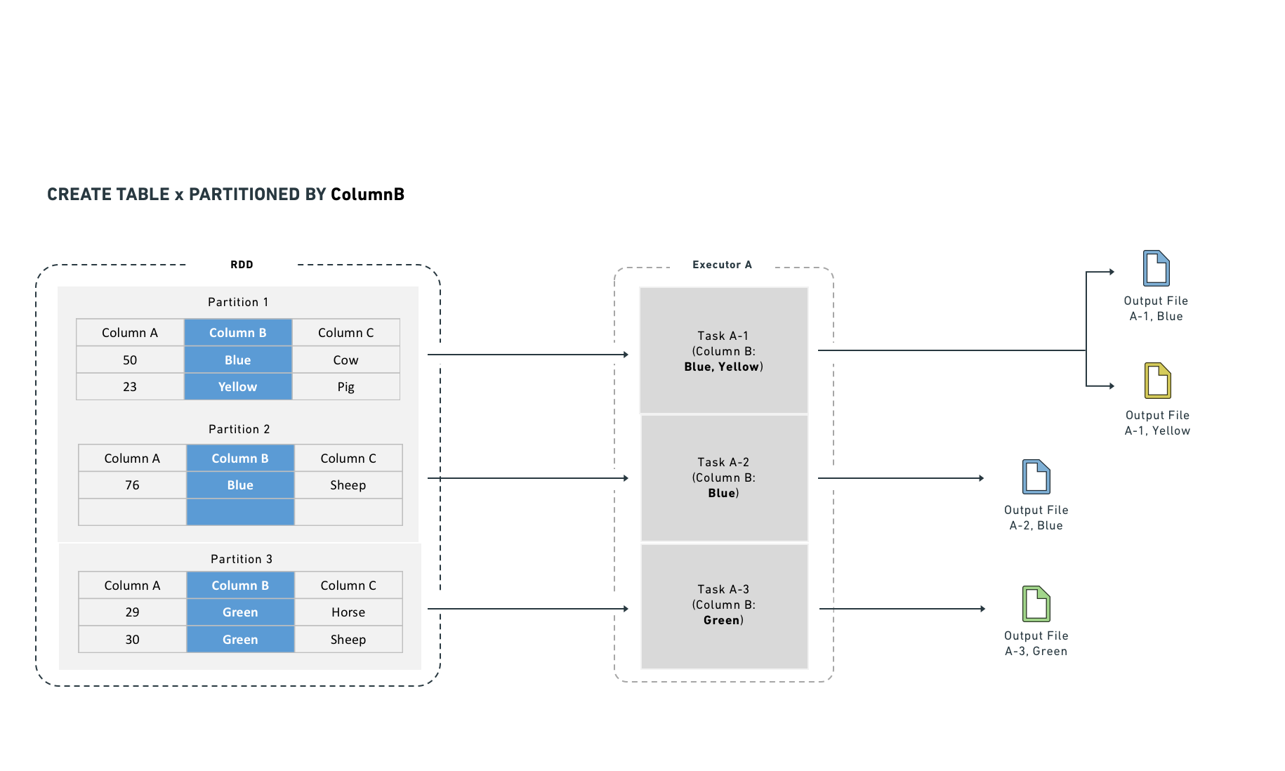
Hive partitioning optimizes partition pruning, filter pushdown, and shuffles. It works best on low-cardinality columns and writes one output file per unique value in each task.

Hive partitioning also integrates with the query planner to make filtering more efficient by reducing the number of files Spark reads. It organizes data into directories named by partition column value. Filter queries can then examine the directory structure to prune files rather than reading data from disk.

For example, if you partition by "year" and "month," Spark lays data out as /path/to/dataset/year=2017/month=09.

This layout allows Spark to read only the files that match a filter (for example, a WHERE clause in SQL). While Hive partitioning can reduce filter-dependent overhead significantly, it also increases the number of output files (at least one per partition). Non-filter operations become less efficient because Spark must read from many files.

Hive partitioning with SparkSQL

:::callout{theme="neutral"} SQL statements that use CREATE TABLE—including the Hive partitioning operation described below—cannot run in Code Workbook. To use SQL, work in a Code Repository with the syntax below. :::

CREATE TABLE `/path/to/output` USING parquet
PARTITIONED BY (a) AS (
SELECT a, b, c
FROM `/path/to/dataset`
CLUSTER BY a
)

The CLUSTER BY command is still necessary, for the same reasons described in the bucketing section.

You can combine CLUSTERED BY and PARTITIONED BY, which generates both subdirectory separation and file-level bucketing. Use caution when combining these options, because the combination can produce a large number of output files.

Example: Partitioning log data

You have log data arriving daily and most queries are time-bounded, so you partition by date:

date=2017-01-01/my_parquet_file0
date=2017-01-02/my_parquet_file1
...
date=2017-01-30/my_parquet_file30

If you query:

SELECT * FROM logs WHERE date < to_date('2017-01-03')

Spark touches only the files under the 2017-01-01 and 2017-01-02 directories. This reduces both the total data read and the number of tasks. The physical plan for a correctly partitioned query looks like this:

*FileScan parquet default.logs[content#158,date#159] Batched: true, Format: Parquet, Location: PrunedInMemoryFileIndex[], PartitionCount: 2, PartitionFilters: [isnotnull(date#159), (date#159 < 17169)], PushedFilters: [], ReadSchema: struct<content:string>

PartitionCount shows the number of Hive partitions that passed the PartitionFilters. These partitions become the input to the FileScan.

As noted above, Hive partitioning uses the same write mechanism as bucketing:

```java tab="Java" DatasetFormatSettings format = DatasetFormatSettings.builder() .addPartitionColumns("date") .build();

output.getDataFrameWriter(df) .setFormatSettings(format) .write();

```python tab="Python"
output.write_dataframe(df, partition_cols=["date"])

``sql tab="SQL" CREATE TABLElogs` USING parquet PARTITIONED BY (date) AS SELECT ...

:::callout{theme="danger"}
Mesa datasets that consume Hive-partitioned data cannot read Hive partition columns correctly; these columns become null values. Do not use Hive partitioning if a direct consumer is a Mesa Transforms dataset.
:::

### Joins

Certain computations require executors to shuffle data so that rows with the same key are co-located. Shuffles consume network I/O and disk I/O, which degrades performance. You can reduce this cost by materializing the join or aggregate as a separate dataset. This approach computes the join once, and subsequent transforms or Contour services reuse the result instead of recomputing it, which avoids repeated shuffle costs.

![Diagram showing how joining and aggregating data before computation eliminates the need for shuffling.](https://palantir.com/docs/resources/foundry/optimizing-pipelines/optimize-join-and-aggregate-example.png)

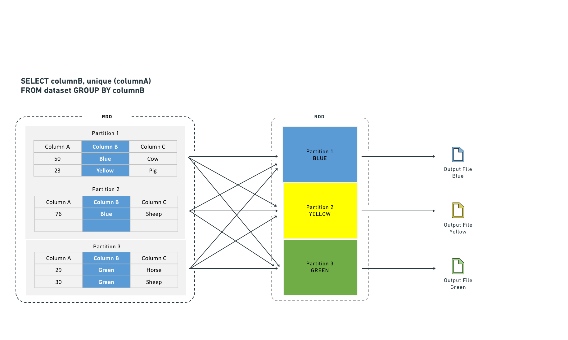
Executors shuffle data to co-locate rows by key for certain computations. Shuffles consume network I/O and disk I/O. Joining and aggregating (then sorting) before computation eliminates the need to shuffle data. This resembles Hive partitioning, but occurs before the task starts rather than after it completes.

Spark supports two join strategies:

* **Sort-merge join (default):** Spark shuffles both sides by join key, sorts each partition, and then merges. This requires both a shuffle and a sort. You can improve sort-merge join performance by bucketing the inputs by join key.
* **Broadcast join:** Spark copies the right-side dataset to every executor before executing the join. Because no row-level shuffle is required, broadcast joins perform faster. However, broadcast joins duplicate the entire right-side dataset to every executor, which increases total memory consumption across the cluster.

A broadcast join copies the right-side dataset to every specified executor before executing the join:

![Diagram showing how broadcasting copies the right side dataset to every executor.](https://palantir.com/docs/resources/foundry/optimizing-pipelines/optimize-broadcast-example.png)

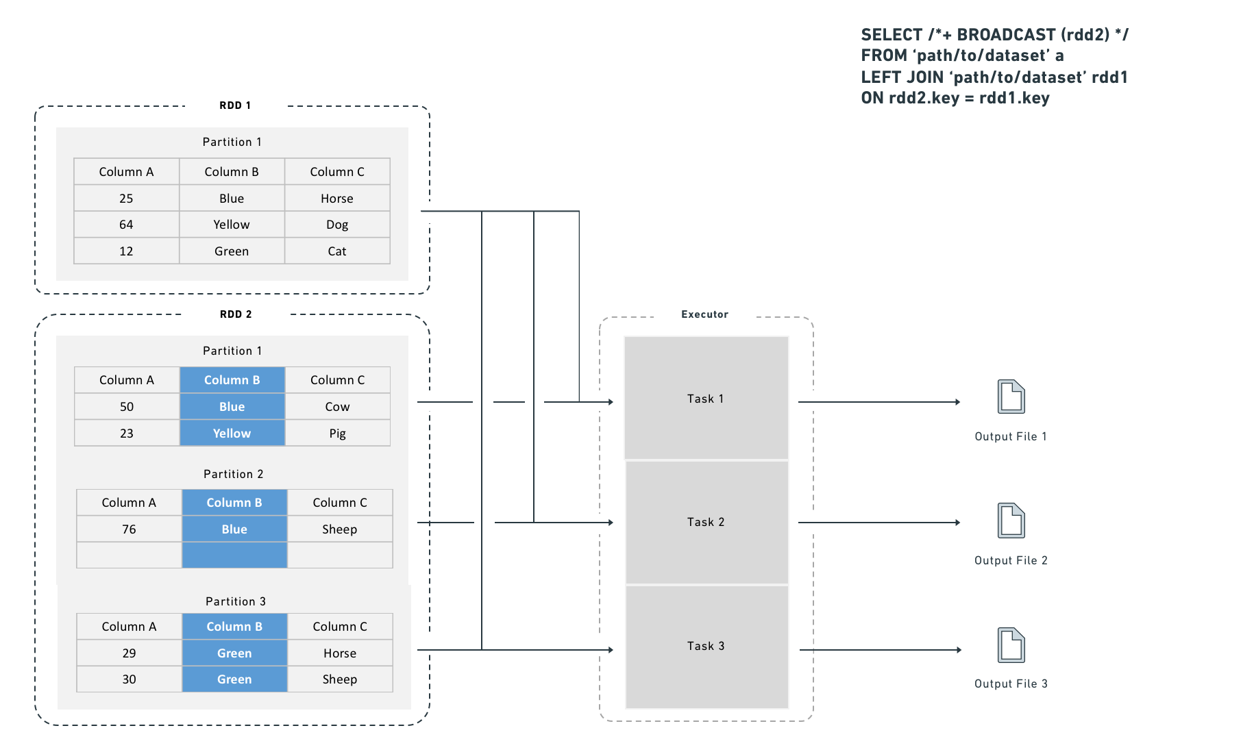
#### Choosing between a shuffle join and a broadcast join

Use a broadcast join when the smaller dataset fits in executor memory (for example, fewer than one million rows). Spark applies broadcast joins automatically based on the `autoBroadcastJoinThreshold` setting, which defaults to 10 MB on disk and is user-configurable. You can also provide explicit hints, which are useful for intermediate results that you know are small (for example, after an aggressive filter or a join that reduces row count).

#### Broadcast join syntax

```python tab="Python"
from pyspark.sql import functions as F

df_a.join(F.broadcast(df_b), df_a["key"] == df_b["key"], "left")

``sql tab="SQL" SELECT /*+ BROADCAST (b) */ * FROMpath/to/dataseta LEFT JOINpath/to/dataset` b ON a.key = b.key

Depending on configuration, Spark may convert a join to a broadcast join automatically for small datasets, even without the hint above.

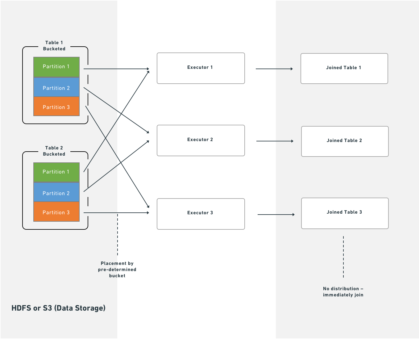
Without bucketing, joins require an extra distribution stage:

![Diagram showing the extra distribution stage when bucketing is not used with joins.](https://palantir.com/docs/resources/foundry/optimizing-pipelines/optimize-joins-without-bucketing-example.png)

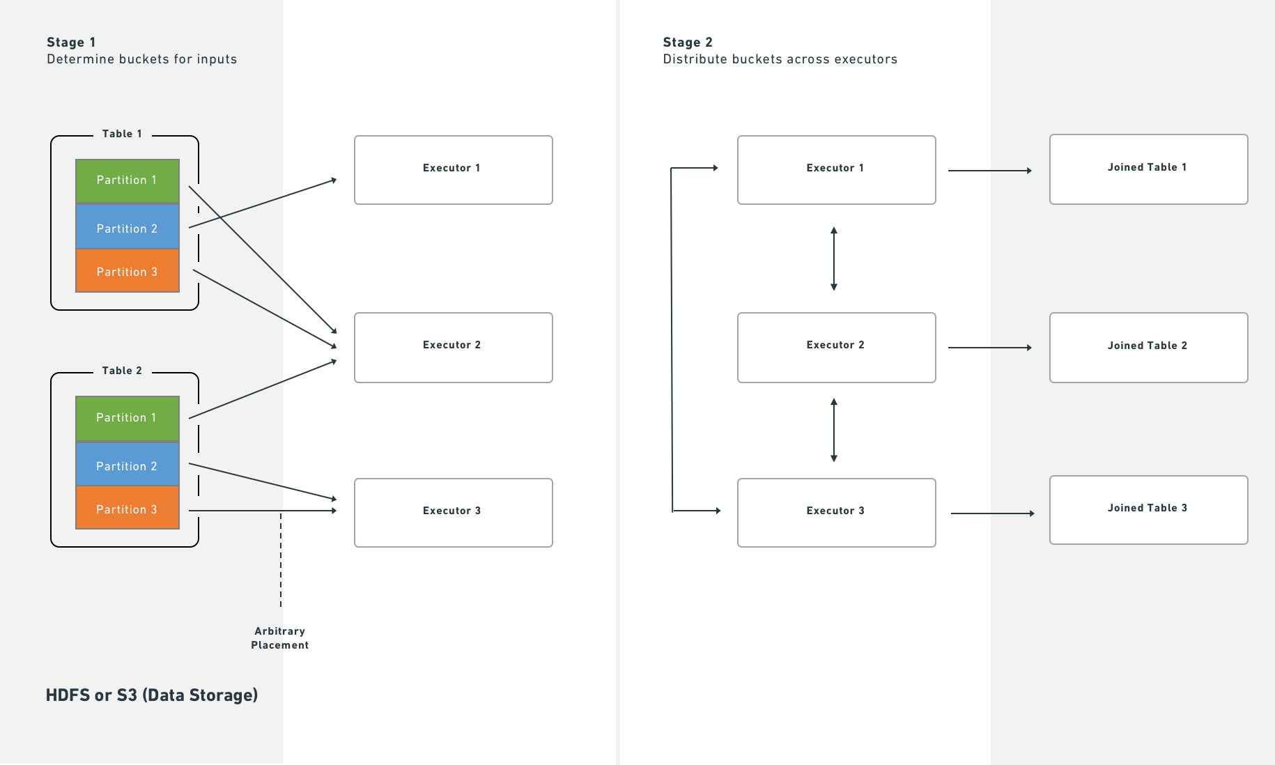
With bucketing, Spark executes joins immediately after reading partitions from HDFS or S3:

![Diagram showing how joins are implemented immediately after reading partitions when bucketing is used.](https://palantir.com/docs/resources/foundry/optimizing-pipelines/optimize-joins-with-bucketing-example.png)

### Splitting the transform

If bucketing, partitioning, and join materialization do not resolve performance issues, consider splitting a single transform into multiple transforms. This approach can clarify the minimal intermediate datasets needed and the most efficient partitioning and bucketing for each step. Note, however, that splitting jobs introduces scheduling and orchestration overhead, so expect some performance penalty.

### Increase resources

**As a last resort**, you can request that Foundry allocates additional resources to your transform. Use [transform metrics](https://palantir.com/docs/foundry/transforms-python/metrics/) to measure and monitor the performance of your pipelines before and after making changes. Exhaust the techniques above before requesting more resources, because:

* Additional resource allocation increases the load on the cluster.
* Spark uses a "fair share" mechanism to reclaim unused resources from other jobs. If multiple transforms over-allocate, they reclaim each other's resources continuously, which adds overhead and reduces performance for all services on the cluster.

Some transformations on large datasets cannot complete in acceptable time without additional resources. If you determine that more resources are necessary, contact Palantir Support to obtain the correct allocation.


---

# 中文翻译

# Spark 优化

本文档介绍了优化 Spark 管道的策略和最佳实践，涵盖了在 Palantir 平台上构建高效管道的基础和高级概念。

## 基本优化

三个核心原则指导基本的 Spark 优化：

| 概念 | 描述 |
| --- | --- |
| 减少数据量 | 尽早过滤掉不需要的行，并删除未使用的列。保持过滤表达式简单且具体。 |
| 重新分区 | 通过调整文件或分区的拆分方式，平衡分区数量与执行器数量。 |
| 清理数据 | 在处理前标准化值。例如，将 `Spark` 和 `spark` 统一为一种大小写格式。Spark 会将不同大小写的字符串视为不同的值。 |

### 减少数据量

提升 Spark 性能的一个直接方法是尽早移除不需要的数据。两种技术有所帮助：

1. 重新排序操作，使过滤、排序步骤和内连接在更早的阶段执行。
2. 删除下游逻辑不需要的列。

:::callout{theme="warning"}
Spark 会严格按照编写的方式执行操作。为避免意外行为，请确保数据已清理和标准化，并且过滤条件针对精确的值。
:::

对 Parquet 元数据进行拆分或排序（Spark 会自动应用）仅当输入数据已经清理和过滤后，才能提升下游性能。

:::callout{theme="neutral"}
低效过滤器的示例有哪些？
在 DataFrame 中使用用户定义函数（UDF），而等效的 DataFrame API 方法已经存在时。
:::

### 为什么减少数据量很重要

尽早过滤并删除未使用的列可以减少每个任务执行的网络 I/O 和磁盘 I/O，从而改善整体作业运行时间。

**操作顺序很重要。** 如果推迟删除不需要的数据直到后期阶段，Spark 会在每个前置阶段处理这些数据。先删除数据可以消除这种开销。请注意，当启用基于成本的优化器时，它会自动处理这种重新排序。

例如，如果 `D` 是一个数据集，你将其与数据集 `SMALL` 和 `BIG` 进行内连接，以下查询：

```sql
SELECT * FROM D JOIN SMALL ON SMALL.key = D.key JOIN BIG ON BIG.key2 = D.key2

性能优于：

SELECT * FROM D JOIN BIG ON BIG.key2 = D.key2 JOIN SMALL ON SMALL.key = D.key

限制 D、BIG 和 SMALL 的列集可以进一步提升性能。请注意，当 Spark 知道 SMALL 和 BIG 的大小时，它会自动尝试将较大的数据集保留在原位。

盲目优化

盲目优化旨在无论具体操作如何，都能提升 Spark 性能。总体目标是使输入分片数量与执行器数量匹配。正确的执行器数量取决于你可用资源和负载。

使用以下近似值来确定分片数量：

结构	分片数量
输入文件支持分片，未分区	分片数量 = 执行器数量 = (文件大小 / HDFS 块大小)
输入文件支持分片，已分区	分片数量 = 执行器数量 = 分区数量
输入文件不支持分片	分片数量 = 执行器数量 = 输入文件数量

在最后一种情况下，当输入文件不支持分片时，Spark 必须在处理文件之前获取组成该文件的所有块。因此，读取开销超过了在 BLOCK_SIZE 下读取单个文件的开销。

在最坏的情况下，盲目优化可能为每个节点分配超出其处理能力的数据，从而导致作业中止。在这种情况下，增加任务数量。请记住，连接操作可能产生比输入数据集总和更大的输出（当连接键匹配多行时）。当进行聚合和连接时，将输入分片与执行器匹配也可能导致问题，因为操作可能产生超出可用内存的组。

当你知道将要运行的操作时，可以应用操作感知优化。这些优化允许你控制分区（或输入分片）的数量，以减少计算期间的洗牌。两种操作感知优化是：1) 分桶 和 2) 分区。

清理数据

Spark 不会从字符串内容推断意图。在内部，Spark 将每个唯一字符串转换为数字标识符，字符串中的任何差异（包括大小写）都会产生单独的标识符。例如，Spark 为 'filter' 分配一个整数，为 'Filter' 分配另一个整数，这使其无法识别两者代表相同的值。为避免此问题，请使字符串过滤区分大小写（例如，同时过滤 'filter' 和 'Filter'），并在处理前清理数据（例如，将所有变体标准化为一致的大小写，不包含额外字符）。

高级优化

上述基本方法是每个管道应执行的最低步骤。当这些方法不足时，本节中的技术可以提供帮助。四个目标指导高级优化：

1. 将数据均匀地或按正确键分布到多个执行器（分区）。
2. 保持任务输入足够小，以适应执行器内存。
3. 减少网络 I/O 和磁盘 I/O，这意味着限制文件数量。
4. 减少任务数量，因为每个任务都会增加调度开销。

七种数据格式化方法可以解决这些目标。哪些方法适用取决于你的工作负载和优先级。

方法	替代术语	描述	影响的步骤	何时使用	何时不使用
基本分区：合并	合并、改变分区数量、DataFrame 分区、数据格式化、重新分区	减少任务之间的分区数量，从而减少总任务数。	步骤 2（RDD 到执行器）	在任务完成后，希望减少输出分区数量时。	当任务没有显著改变数据量时。
基本分区：按值重新分区	重新分区、DataFrame 分区、数据格式化、按键分区	计算后，根据特定列值（例如名称或 ID）将行重新分配到新分区。	步骤 2（RDD 到执行器）	当分区列具有少量不同值（低基数）时。	当分区列具有许多不同值（大约大于 1,000）时。
哈希分区	分桶（和排序）	基于元数据在 RDD 中创建排序分区。输出文件使用桶标识符（output.bucket1.parquet）而不是值名称。	步骤 3（执行器到输出文件）	当下游计算匹配行键（聚合、连接）或预排序对多个用例有益时。	当没有明确的下游收益时。仅在你有特定性能目标时使用分桶。
Hive 分区	动态分区、分区	计算后，将结果拆分为按分区键组织的输出文件，存储在按每个键值命名的子目录中。	步骤 3（执行器到输出文件）	大型数据集，具有低基数列，且过滤剪枝能提供显著收益时。	当结果会产生过多小文件时。
连接和聚合	—	物化连接或聚合的数据集，以便下游转换和服务重用，而不是重新计算连接。	不适用	当多个下游消费者重复连接这些数据集时（例如在 Contour 中）。	当未过滤的连接数据集过大，或连接运行频率低且额外管道步骤损害整体性能时。
拆分转换	—	将单个转换拆分为多个转换，以隔离中间步骤。	不适用	当其他技术失败，或单独步骤有助于调试和管理，或需要持久化中间状态时。	当上述技术已提供足够性能时。
增加资源	—	为你的转换分配额外的 Foundry 资源。为一个转换增加资源会增加集群负载，并可能降低其他服务的性能。	所有步骤	作为最后手段，仅当没有其他选项能产生可接受性能且你有紧急需求时。	在所有其他情况下。

基本分区：合并（改变分区数量）

合并接受目标分区数量，并在单个任务内顺序处理多个输入分区。

优点： 当你有大量大致均匀分布的数据（例如 TB 级）时，合并效果良好。它避免了在集群中重新分布数据的成本。

缺点： 合并不会重新分布数据，因此输出任务的大小可能不均匀。

```java tab="Java" df.coalesce(N);

```python tab="Python"
df.coalesce(N)

SQL 不支持此操作。

基本分区：按值重新分区

按值重新分区类似于合并，但它对每行进行哈希处理，并将数据均匀分布到集群中。

优点： 产生均匀分布的数据，从而产生更可预测的文件大小。

缺点： Spark 将数据集写入临时空间并通过网络传输。此成本随数据集大小增长，因此当重新分布开销超过收益时，避免重新分区大型数据集。

```java tab="Java" df.repartition(N);

```python tab="Python"
df.repartition(N)

SQL 不支持此操作。

在 SparkSQL 中，你也可以按给定列集重新分区，这会哈希这些列而不是整行。此技术将在后续章节中讨论。请注意，基于列的重新分区不会在 Spark 查询计划器读取输出文件时通知它。

```java tab="Java" df.repartition(N, "column1");

```python tab="Python"
df.repartition(N, "column1")

```sql tab="SQL" DISTRIBUTE BY column1

### 哈希分区（分桶和排序）

上述基本分区方法是改善管道性能的首选技术。然而，由于 Palantir 在整个过程中使用 SparkSQL，你可以通过以有利于 SparkSQL 查询计划器的格式写入数据集来进一步扩展优化。SparkSQL 允许你写入描述数据集如何分区以及每个分区内排序顺序的元数据，然后它可以利用这些元数据跳过下游的昂贵操作。两种方法提供此功能：1) 分桶（和排序）和 2) Hive 分区。

**分桶** 按键将行分组到输出文件中，从而加速跨行匹配键的计算（连接、分组操作）。当你有多个输入时，对所有输入进行分桶以获得最佳结果。分桶类似于分区，但每个分区放置多个值而不是单个值。选择正确的桶数量需要平衡多个约束——目标是创建满足以下条件的文件：

* 适合每个节点（以利用可用空间）而不超过节点容量（以避免崩溃）
* 不小于 HDFS 块大小
* 遵循分区到任务到执行器的一对一原则（除非与前述约束冲突）

:::callout{theme="neutral"}
分桶和排序对大型数据集有益，但在应用之前必须了解或控制数据分布。单独分桶有帮助，但结合分桶和排序能获得最佳结果。
:::

一般建议是目标输出文件（桶）大小为 128–512 MB。如果你执行大量大型连接，可能需要调整这些目标。

即使输入分区为 128 MB，计算也可能扩展数据。128 MB 的输入分区可能产生 512 MB 的输出文件。

#### 使用 SparkSQL 进行分桶

:::callout{theme="neutral"}
使用 `CREATE TABLE` 的 SQL 语句——包括下面描述的分桶和排序操作——不能在 Code Workbook 中运行。要使用 SQL 进行分桶，请使用以下语法的 Code Repository。
:::

```sql
CREATE TABLE `/path/to/output` USING parquet
CLUSTERED BY (a)
SORTED BY (a)
INTO 200 BUCKETS AS (
SELECT a, b, c
FROM `/path/to/dataset`
CLUSTER BY a
)

上述查询使用了两个不同的 SQL 命令，它们服务于不同的目的：

• CLUSTERED BY（和 SORTED BY）修改 CREATE TABLE 语句以指定表的物理布局。这些关键字控制实际的分桶到单独文件。
• CLUSTER BY 是一个数据操作，触发洗牌，以便集群内的任务按指定键分组数据。这一步通常是必要的，因为每个 Spark 任务和执行器独立运行。没有 CLUSTER BY，每个任务仅对其自身执行器内存中的数据进行分桶。

示例：为什么 CLUSTER BY 很重要

考虑一个案例，有 200 个最终任务，按一个具有 200 个可能值的键进行分桶。没有 CLUSTER BY，这 200 个值均匀分布在所有 200 个任务中。每个任务为其遇到的每个键值创建一个文件，产生 200 × 200 = 40,000 个文件。此文件数量会导致下一个管道步骤的读取开销急剧增加。

如果你知道每个任务已经拥有与分桶键几乎一对一关系的数据（例如，在 GROUP BY 之后），可以省略 CLUSTER BY。省略它可以节省一次洗牌，但请仔细监控输出文件的数量。

注意： Spark 的 SQL 接口并不总是产生预期的结果（即每个桶一个文件）。如果你无法调整 SQL 以达到期望的输出，请改用 Python。

numPartitions 控制输出文件的数量。shuffle 参数强制在文件间重新平衡数据。如果你的输入已经良好平衡，将 shuffle 设置为 false 以提升性能。如果你的输入不平衡——或者转换造成不平衡（例如，仅匹配某些输入文件中行的过滤器）——将 shuffle 设置为 true。

在 Python 中，两种方法对应于洗牌/无洗牌选项。无洗牌等效项（shuffle: false）：

df.coalesce(N)

洗牌等效项（shuffle: true）：

df.repartition(N)

示例：对索赔数据集进行分桶

你有一个 claims 数据集，你的大部分分析涉及对给定 patient_id 的窗口函数、在 patient_id 上连接以引入参考数据，或聚合。

默认情况下，此查询：

SELECT claims.patient_id, age FROM claims LEFT JOIN patients on claims.patient_id = patients.patient_id

产生此物理计划：

== Physical Plan ==*Project [patient_id#50, age#52]+- SortMergeJoin [patient_id#50], [patient_id#51], LeftOuter:- *Sort [patient_id#50 ASC NULLS FIRST], false, 0:  +- Exchange hashpartitioning(patient_id#50, 200):     +- *FileScan parquet default.claims[patient_id#50] Batched: true, Format: Parquet, Location: InMemoryFileIndex[file:/Volumes/git/spark/spark-warehouse/claims], PartitionFilters: [], PushedFilters: [], ReadSchema: struct<patient_id:string>+- *Sort [patient_id#51 ASC NULLS FIRST], false, 0+- Exchange hashpartitioning(patient_id#51, 200)+- *FileScan parquet default.patients[patient_id#51,age#52] Batched: true, Format: Parquet, Location: InMemoryFileIndex[file:/Volumes/git/spark/spark-warehouse/patients], PartitionFilters: [], PushedFilters: [], ReadSchema: struct<patient_id:string,age:int>

每个 FileScan 后的 Exchange 表示 Spark 按 patient_id 将表洗牌到 200 个分区，对每个分区按 patient_id 排序，然后执行 SortMergeJoin。对于 100 GB 的 claims 和 1 GB 的 patients，这会产生一个资源密集型作业，因为 Spark 必须将所有数据重新分布到集群中。

你可以通过使用分桶元数据重写 claims 和 patients，用写入时间成本换取更快的读取时间：

```java tab="Java" DatasetFormatSettings format = DatasetFormatSettings.builder() .numBuckets(200) .addBucketColumns("patient_id") .addSortColumns("patient_id") .build();

output.getDataFrameWriter(df) .setFormatSettings(format) .write();

```python tab="Python (Code Repository)"
output.write_dataframe(df,bucket_cols=["patient_id"],bucket_count=200,sort_by=["patient_id"])

```python tab="Python (Code Workbook)" from vector.api import DataFrameReturn

def my_vector_node(my_input): return DataFrameReturn(my_input, bucket_cols=["patient_id"], bucket_count=200, sort_by=["patient_id"])

```sql tab="SQL"
CREATE TABLE `claims` USING parquet
CLUSTERED BY (patient_id)
SORTED BY (patient_id)
INTO 200 BUCKETS AS
SELECT ...

相同的查询现在产生此物理计划：

== Physical Plan ==*Project [patient_id#72, age#73]+- SortMergeJoin [patient_id#72], [patient_id#75], LeftOuter:- *FileScan parquet default.claims[patient_id#72,age#73] Batched: true, Format: Parquet, Location: InMemoryFileIndex[file:/Volumes/git/spark/spark-warehouse/claims], PartitionFilters: [], PushedFilters: [], ReadSchema: struct<patient_id:string,age:int>+- *FileScan parquet default.patients[patient_id#75] Batched: true, Format: Parquet, Location: InMemoryFileIndex[file:/Volumes/git/spark/spark-warehouse/patients], PartitionFilters: [], PushedFilters: [], ReadSchema: struct<patient_id:string>

由于 Foundry 存储了关于分桶和排序的元数据，Spark 在从 HDFS 或 S3 获取数据后立即开始连接。这消除了洗牌和排序阶段，从而减少了作业运行时间。不会发生本地磁盘写入，除了初始获取外也不需要额外的网络流量。

分桶如何影响写入端

分桶和排序不会改变转换本身——它们仅控制作业的最终任务如何写入输出。使用 claims 示例：Spark 不是将输出数据顺序写入单个文件，而是创建一个临时列 bucket，定义为 hash(patient_id) % 200，然后在分区内按 (bucket, patient_id) 排序。如果你的输入数据如下所示：

A
C
A
A
B
C

Spark 将其格式化为（假设 A 和 B 哈希到 0，C 哈希到 1）：

0 A
0 A
0 A
0 B
1 C
1 C

然后 Spark 扫描分区并为每个桶值写入一个单独的文件——在此例中是两个文件。

如果你在写入前立即运行 repartition(200, "patient_id")，每个任务会产生一个文件，因为桶值在每个任务内是恒定的。然而，对于均匀分布的数据，最坏情况是每个任务写入 200 个单独文件。对于 200 个输出任务，这会产生 40,000 个输出文件，这会降低写入和读取性能。高文件数量也会影响 Foundry Catalog 和 Cassandra 性能，因此请尽可能限制输出文件的数量。

Hive 分区

"分区"在 Spark 中是一个过载的术语。文档通常使用标签"Hive 风格"、"目录"或"动态"分区来区分此变体。

Hive 分区 发生在第三步。Apache Hive 是一个在分布式计算环境中存储、查询和分析大型数据集的系统。

Hive 分区以与分桶相同的方式写入数据，但向输出排序添加了一个分区列。Spark 使用此列将数据组织到子目录中——它为分区列中的每个唯一值至少产生一个输出文件。因此，对低基数列（具有许多重复值的列）使用 Hive 分区，其中过滤剪枝能提供可衡量的收益。

:::callout{theme="neutral"} 与分桶一样，如果不小心，Hive 分区可能产生过多小文件。 :::

:::callout{theme="neutral"} 分桶和 Hive 分区都打破了一对一原则。它们要么输出与任务数量不同的文件，要么重新排列每个任务写入的数据，因此结果不一定是每个任务一个输出文件。 :::

Hive 分区优化了分区剪枝、过滤器下推和洗牌。它在低基数列上效果最佳，并在每个任务中为每个唯一值写入一个输出文件。

Hive 分区还与查询计划器集成，通过减少 Spark 读取的文件数量使过滤更高效。它将数据组织到按分区列值命名的目录中。过滤查询随后可以检查目录结构以剪枝文件，而不是从磁盘读取数据。

例如，如果你按"year"和"month"分区，Spark 将数据布局为 /path/to/dataset/year=2017/month=09。

此布局允许 Spark 仅读取与过滤器匹配的文件（例如 SQL 中的 WHERE 子句）。虽然 Hive 分区可以显著减少依赖过滤器的开销，但它也增加了输出文件的数量（每个分区至少一个）。非过滤器操作变得效率较低，因为 Spark 必须从许多文件中读取。

使用 SparkSQL 进行 Hive 分区

:::callout{theme="neutral"} 使用 CREATE TABLE 的 SQL 语句——包括下面描述的 Hive 分区操作——不能在 Code Workbook 中运行。要使用 SQL，请使用以下语法的 Code Repository。 :::

CREATE TABLE `/path/to/output` USING parquet
PARTITIONED BY (a) AS (
SELECT a, b, c
FROM `/path/to/dataset`
CLUSTER BY a
)

CLUSTER BY 命令仍然是必要的，原因与分桶部分所述相同。

你可以组合 CLUSTERED BY 和 PARTITIONED BY，这会同时生成子目录分离和文件级分桶。组合这些选项时请谨慎，因为组合可能产生大量输出文件。

示例：对日志数据进行分区

你有每天到达的日志数据，大多数查询是时间受限的，因此你按日期分区：

date=2017-01-01/my_parquet_file0
date=2017-01-02/my_parquet_file1
...
date=2017-01-30/my_parquet_file30

如果你查询：

SELECT * FROM logs WHERE date < to_date('2017-01-03')

Spark 仅触及 2017-01-01 和 2017-01-02 目录下的文件。这减少了总读取数据量和任务数量。正确分区查询的物理计划如下所示：

*FileScan parquet default.logs[content#158,date#159] Batched: true, Format: Parquet, Location: PrunedInMemoryFileIndex[], PartitionCount: 2, PartitionFilters: [isnotnull(date#159), (date#159 < 17169)], PushedFilters: [], ReadSchema: struct<content:string>

PartitionCount 显示通过 PartitionFilters 的 Hive 分区数量。这些分区成为 FileScan 的输入。

如上所述，Hive 分区使用与分桶相同的写入机制：

```java tab="Java" DatasetFormatSettings format = DatasetFormatSettings.builder() .addPartitionColumns("date") .build();

output.getDataFrameWriter(df) .setFormatSettings(format) .write();

```python tab="Python"
output.write_dataframe(df, partition_cols=["date"])

``sql tab="SQL" CREATE TABLElogs` USING parquet PARTITIONED BY (date) AS SELECT ...

:::callout{theme="danger"}
消费 Hive 分区数据的 Mesa 数据集无法正确读取 Hive 分区列；这些列会变为空值。如果直接消费者是 Mesa Transforms 数据集，请不要使用 Hive 分区。
:::

### 连接

某些计算要求执行器洗牌数据，以便具有相同键的行共置。洗牌消耗网络 I/O 和磁盘 I/O，从而降低性能。你可以通过将连接或聚合物化为单独数据集来减少此成本。此方法计算一次连接，后续转换或 Contour 服务重用结果而不是重新计算，从而避免重复的洗牌成本。

![显示在计算前连接和聚合数据如何消除洗牌需求的图表。](https://palantir.com/docs/resources/foundry/optimizing-pipelines/optimize-join-and-aggregate-example.png)

执行器洗牌数据以按键共置行用于某些计算。洗牌消耗网络 I/O 和磁盘 I/O。在计算前连接和聚合（然后排序）消除了洗牌数据的需要。这类似于 Hive 分区，但发生在任务开始之前而不是完成之后。

Spark 支持两种连接策略：

* **排序合并连接（默认）：** Spark 按连接键洗牌两侧，对每个分区排序，然后合并。这需要洗牌和排序。你可以通过按连接键对输入进行分桶来改善排序合并连接的性能。
* **广播连接：** Spark 在执行连接前将右侧数据集复制到每个执行器。由于不需要行级洗牌，广播连接执行更快。然而，广播连接将整个右侧数据集复制到每个执行器，这增加了集群中的总内存消耗。

广播连接在执行连接前将右侧数据集复制到每个指定执行器：

![显示广播如何将右侧数据集复制到每个执行器的图表。](https://palantir.com/docs/resources/foundry/optimizing-pipelines/optimize-broadcast-example.png)

#### 在洗牌连接和广播连接之间选择

当较小的数据集适合执行器内存时（例如，少于一百万行），使用广播连接。Spark 基于 `autoBroadcastJoinThreshold` 设置自动应用广播连接，该设置默认为磁盘上 10 MB，并且可由用户配置。你也可以提供显式提示，这对于你知道很小的中间结果很有用（例如，在激进过滤或减少行数的连接之后）。

#### 广播连接语法

```python tab="Python"
from pyspark.sql import functions as F

df_a.join(F.broadcast(df_b), df_a["key"] == df_b["key"], "left")

sql tab="SQL" SELECT /*+ BROADCAST (b) */ * FROM `path/to/dataset` a LEFT JOIN `path/to/dataset` b ON a.key = b.key

根据配置，即使没有上述提示，Spark 也可能自动将小数据集的连接转换为广播连接。

没有分桶时，连接需要额外的分布阶段：

使用分桶时，Spark 在从 HDFS 或 S3 读取分区后立即执行连接：

拆分转换

如果分桶、分区和连接物化未能解决性能问题，考虑将单个转换拆分为多个转换。此方法可以澄清所需的最小中间数据集以及每个步骤最有效的分区和分桶。然而，请注意，拆分作业会引入调度和编排开销，因此预期会有一些性能损失。

增加资源

作为最后手段，你可以请求 Foundry 为你的转换分配额外资源。使用转换指标在更改前后测量和监控管道的性能。在请求更多资源之前，请用尽上述技术，因为：

• 额外资源分配会增加集群负载。
• Spark 使用"公平共享"机制从其他作业回收未使用的资源。如果多个转换过度分配，它们会持续回收彼此的资源，这会增加开销并降低集群上所有服务的性能。

一些对大型数据集的转换在没有额外资源的情况下无法在可接受的时间内完成。如果你确定需要更多资源，请联系 Palantir 支持以获得正确的分配。