Visualize data（可视化数据）

In Code Workbook, you can use open-source visualization libraries to display visualizations of your data. These visualizations can then be shared with others, for instance in Notepad documents.

Python Visualizations

In Python, Code Workbook supports visualizations using Matplotlib, Seaborn, and Plotly.

Using Matplotlib and Seaborn

When using Matplotlib, a call to matplotlib.pyplot.show() causes the resulting plot image to be saved in the transform output and returned to the user interface, allowing the creation of customized plots. As with any visualization, you can download this image by right-clicking the transform in the graph and choosing Download image.

Here is an example of a transform that uses Matplotlib to render a visualization:

def viz_plot_univariate_distribution_using_histogram(input_dataset):
    import matplotlib.mlab as mlab
    import matplotlib.pyplot as plt

    INPUT_DF = input_dataset
    SELECTED_COLUMN = "column_to_plot" # Note this should be a numeric column
    NUM_BINS = number_of_bins

    # Histogram the selected column
    bins, counts = INPUT_DF.select(SELECTED_COLUMN).rdd.flatMap(lambda x:x).histogram(NUM_BINS)

    # Plot the histogram
    fig, ax = plt.subplots()
    ax.hist(bins[:-1], bins, weights=counts, density=True)

    ax.set_xlabel(SELECTED_COLUMN)
    ax.set_ylabel('Probability density')
    ax.set_title(r'Histogram of ' + str(SELECTED_COLUMN))

    # Tweak spacing to prevent clipping of ylabel
    fig.tight_layout()
    plt.show()

When using Seaborn, a data visualization library based on Matplotlib, you must call matplotlib.pyplot.show() to return the image to the frontend.

You can add Seaborn to your environment by editing your profile or by customizing your workbook's environment.

def seaborn_example(pandas_df):
    import seaborn as sns
    import matplotlib.pyplot as plt

    sns.set_theme()

    # Create a visualization
    sns.relplot(
        data=pandas_df,
        x="price", y="minimum_nights"
    )

    # This is necessary to capture the plot
    plt.show()

def seaborn_violinplot(pandas_df):
    import seaborn as sns
    import matplotlib.pyplot as plt

    sns.violinplot(x="col_A", y="col_B", data=pandas_df);
    plt.show()

By default, the output of Matplotlib and Seaborn visualizations in Code Workbook will be in PNG format. To output Matplotlib and Seaborn visualizations in SVG format, use the following code before your plot:

set_output_image_type('svg')

Or, use a hint for better visibility:

@output_image_type('svg')
def chart(input):
    # create chart here

Plotting with different languages and fonts using Matplotlib

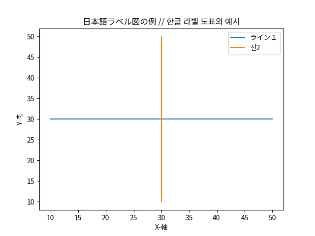
To plot labels and text in languages using non-Roman characters (such as Japanese or Korean) or in non-default fonts using Matplotlib, you must specifically specify which font family you would like Matplotlib to use when rendering images. For more information, refer to the list of available fonts installed by default.

Here is an example of how to specify fonts for Matplotlib:

def japanese_korean_matplotlib_example():
    import matplotlib.mlab as mlab
    import matplotlib.pyplot as plt
    from matplotlib import rcParams
    # Set font family to the Noto Sans CJK font pack
    rcParams['font.family'] = 'Noto Sans CJK JP'
    # create data
    x = [10,20,30,40,50]
    y = [30,30,30,30,30]

    # plot lines
    plt.plot(x, y, label = "ライン１")
    plt.plot(y, x, label = "선2")
    plt.xlabel("X-軸")
    plt.ylabel("Y-축")
    plt.legend()
    plt.title("日本語ラベル図の例 // 한글 라벨 도표의 예시")
    plt.show()

:::callout{title="Matplotlib 2.* Font Designation"} For Matplotlib 2.*, .ttc font files are not detected by Matplotlib automatically. Either upgrade to 3.* or directly add the font filepath to Matplotlib's font manager.

from matplotlib import rcParams
import matplotlib.font_manager as fm
fm.fontManager.ttflist += fm.createFontList(["/usr/share/fonts/opentype/noto/NotoSansCJK-Regular.ttc"])
rcParams['font.family'] = 'Noto Sans CJK JP'</pre>

:::

Using Plotly

Plotly is a visualization library that allows you to create interactive images. To use Plotly, first make sure it is included in your environment.

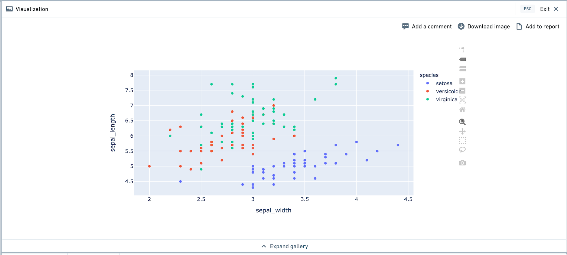
A call to fig.show() causes the resulting plot image to be saved as part of the transform output and returned to the user interface. Here is an example of a transform that uses Plotly to render a visualization, using Plotly Express. Plotly Express comes pre-loaded with the iris dataset.

def plotly_example():
    import plotly.express as px
    df = px.data.iris()
    fig = px.scatter(df, x = "sepal_width", y = "sepal_length", color = "species")
    fig.show()

After running the transform, the Plotly visualization will appear in the visualization tab. We recommend viewing the visualization in full screen mode. You are able to use functionality like zooming in and out, selection on the graph, and so on.

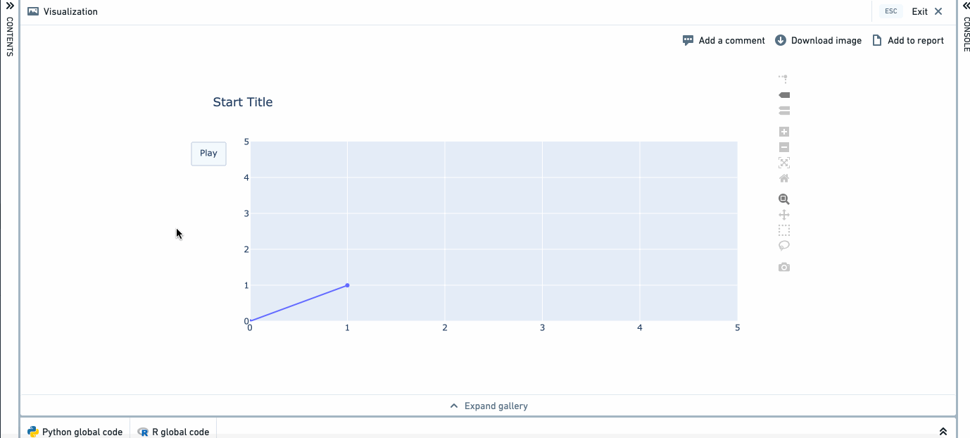
Here is a more complex example, which produces an animated visualization.

def plotly_example_2():
    import plotly.graph_objects as go
    fig = go.Figure(
        data=[go.Scatter(x=[0, 1], y=[0, 1])],
        layout=go.Layout(
            xaxis=dict(range=[0, 5], autorange=False),
            yaxis=dict(range=[0, 5], autorange=False),
            title="Start Title",
            updatemenus=[dict(
                type="buttons",
                buttons=[dict(label="Play",
                          method="animate",
                          args=[None])])]
        ),
        frames=[go.Frame(data=[go.Scatter(x=[1, 2], y=[1, 2])]),
            go.Frame(data=[go.Scatter(x=[1, 4], y=[1, 4])]),
            go.Frame(data=[go.Scatter(x=[3, 4], y=[3, 4])],
                     layout=go.Layout(title_text="End Title"))]
        )

    fig.show()

R Visualizations

In R, Code Workbook supports visualizations using ggplot2 and plotly.

Using ggplot2

fare_distribution <- function(titanic_dataset) {
    hist(titanic_dataset$Fare)
    return(titanic_dataset)
}

example_ggplot <- function() {
    library(ggplot2)
    theme_set(theme_bw())  # pre-set the bw theme
    data("midwest", package = "ggplot2")

    # Scatterplot
    gg <- ggplot(midwest, aes(x=area, y=poptotal)) +
        geom_point(aes(col=state, size=popdensity)) +
        geom_smooth(method="loess", se=F) +
        xlim(c(0, 0.1)) +
        ylim(c(0, 500000)) +
        labs(subtitle="Area Vs Population",
            y="Population",
            x="Area",
            title="Scatterplot",
            caption = "Source: midwest")

    plot(gg)
    return(NULL)
}

By default, ggplot visualizations will be outputted as PNGs. To produce R ggplot visualizations in SVG format, add a hint using a comment:

fare_distribution <- function(titanic_dataset) {
    # image: svg
    hist(titanic_dataset$Fare)
    return(titanic_dataset)
}

To customize the PNG or SVG output, you can call the png() or svg() function using the built-in graphicsFile variable as filename.

unnamed_1 <- function() {
    png(
      filename=graphicsFile,
      width=800,
      height=400,
      units="px",
      pointsize=4,
      bg="white",
      res=300,
      type="cairo")

    plot(1:10, 1:10)
}

Note that if you want to use a custom svg() function, you'll also need to provide a comment hint described above.

unnamed_1 <- function() {
    # image: svg
    svg(
      filename=graphicsFile,
      width=5,
      height=9,
      pointsize=4,
      bg="white")

    plot(1:10, 1:10)
}

Using Plotly

Plotly ↗ allows you to make interactive graphs. To use Plotly in R, add the r-plotly package to your environment. Plot graphs with plot() or print() to show them on the frontend. Here's a simple example:

plotly_example <- function() {
    library(plotly)

    scatter_plotly <- plot_ly (
        x = rnorm(1000),
        y = rnorm(1000),
        mode = "markers",
        type = "scatter"
    )
    plot(scatter_plotly)
}

Plotly limitations

The following notes apply to both Python and R.

• In the console, Plotly visualizations will be converted to images and displayed as PNGs. They will not be interactive. To view an interactive visualization, write the code in a transform.
• When creating Plotly visualizations, visualizations with more than 20,000 points are not recommended due to degraded browser performance. If creating a scatterplot with a large number of points, use scattergl for better performance.

Matplotlib limitations

The following limitations on Matplotlib apply to Python.

• Matplotlib is not thread safe. ↗
• When running multiple nodes, Spark will run these computations in parallel. As a result, unintended behavior may be revealed in the form of Matplotlib Runtime Exceptions or visualizations created in incorrect nodes.
• When using multiple Matplotlib visualizations in separate nodes within a single Code Workbook, you must lock each node. You can lock each node with the thread-safe decorator @synchronous_node_execution, as shown below.

import matplotlib.mlab as mlab
import matplotlib.pyplot as plt
from matplotlib import rcParams
@synchronous_node_execution
def thread_safe_node():
    # Set font family to the Noto Sans CJK font pack
    rcParams['font.family'] = 'Noto Sans CJK JP'
    # create data
    x = [10,20,30,40,50]
    y = [30,30,30,30,30]

    # plot lines
    plt.plot(x, y, label = "ライン１")
    plt.plot(y, x, label = "선2")
    plt.xlabel("X-軸")
    plt.ylabel("Y-축")
    plt.legend()
    plt.title("日本語ラベル図の例 // 한글 라벨 도표의 예시")
    plt.show()

---

中文翻译

可视化数据

在代码工作簿(Code Workbook)中，您可以使用开源可视化库来展示数据的可视化图表。这些可视化结果可以与他人共享，例如在记事本文档中。

Python 可视化

在 Python 中，代码工作簿(Code Workbook)支持使用 Matplotlib、Seaborn 和 Plotly 进行可视化。

使用 Matplotlib 和 Seaborn

使用 Matplotlib 时，调用 matplotlib.pyplot.show() 会将生成的图表图像保存在转换输出中并返回给用户界面，从而支持创建自定义图表。与任何可视化一样，您可以通过右键点击图表中的转换并选择下载图像来下载此图像。

以下是一个使用 Matplotlib 渲染可视化的转换示例：

def viz_plot_univariate_distribution_using_histogram(input_dataset):
    import matplotlib.mlab as mlab
    import matplotlib.pyplot as plt

    INPUT_DF = input_dataset
    SELECTED_COLUMN = "column_to_plot" # 注意：这应为数值列
    NUM_BINS = number_of_bins

    # 对选定列进行直方图统计
    bins, counts = INPUT_DF.select(SELECTED_COLUMN).rdd.flatMap(lambda x:x).histogram(NUM_BINS)

    # 绘制直方图
    fig, ax = plt.subplots()
    ax.hist(bins[:-1], bins, weights=counts, density=True)

    ax.set_xlabel(SELECTED_COLUMN)
    ax.set_ylabel('概率密度')
    ax.set_title(r'直方图 - ' + str(SELECTED_COLUMN))

    # 调整间距以防止 y 轴标签被裁剪
    fig.tight_layout()
    plt.show()

使用基于 Matplotlib 的数据可视化库 Seaborn 时，必须调用 matplotlib.pyplot.show() 才能将图像返回给前端。

您可以通过编辑配置文件或自定义工作簿环境将 Seaborn 添加到您的环境中。

def seaborn_example(pandas_df):
    import seaborn as sns
    import matplotlib.pyplot as plt

    sns.set_theme()

    # 创建可视化
    sns.relplot(
        data=pandas_df,
        x="price", y="minimum_nights"
    )

    # 必须调用以捕获图表
    plt.show()

def seaborn_violinplot(pandas_df):
    import seaborn as sns
    import matplotlib.pyplot as plt

    sns.violinplot(x="col_A", y="col_B", data=pandas_df);
    plt.show()

默认情况下，代码工作簿(Code Workbook)中 Matplotlib 和 Seaborn 可视化的输出格式为 PNG。要以 SVG 格式输出 Matplotlib 和 Seaborn 可视化，请在绘图前使用以下代码：

set_output_image_type('svg')

或者，使用提示(hint)以获得更好的可见性：

@output_image_type('svg')
def chart(input):
    # 在此创建图表

使用 Matplotlib 绘制不同语言和字体

要使用非罗马字符的语言（如日语或韩语）或非默认字体绘制标签和文本，您必须明确指定 Matplotlib 在渲染图像时应使用的字体系列。更多信息，请参考默认安装的可用字体列表。

以下是如何为 Matplotlib 指定字体的示例：

def japanese_korean_matplotlib_example():
    import matplotlib.mlab as mlab
    import matplotlib.pyplot as plt
    from matplotlib import rcParams
    # 将字体系列设置为 Noto Sans CJK 字体包
    rcParams['font.family'] = 'Noto Sans CJK JP'
    # 创建数据
    x = [10,20,30,40,50]
    y = [30,30,30,30,30]

    # 绘制线条
    plt.plot(x, y, label = "ライン１")
    plt.plot(y, x, label = "선2")
    plt.xlabel("X-軸")
    plt.ylabel("Y-축")
    plt.legend()
    plt.title("日本語ラベル図の例 // 한글 라벨 도표의 예시")
    plt.show()

:::callout{title="Matplotlib 2.* 字体指定"} 对于 Matplotlib 2.*，.ttc 字体文件不会被 Matplotlib 自动检测到。请升级到 3.* 或直接将字体文件路径添加到 Matplotlib 的字体管理器中。

from matplotlib import rcParams
import matplotlib.font_manager as fm
fm.fontManager.ttflist += fm.createFontList(["/usr/share/fonts/opentype/noto/NotoSansCJK-Regular.ttc"])
rcParams['font.family'] = 'Noto Sans CJK JP'</pre>

:::

使用 Plotly

Plotly 是一个可视化库，允许您创建交互式图像。要使用 Plotly，首先确保它已包含在您的环境中。

调用 fig.show() 会将生成的图表图像保存为转换输出的一部分并返回给用户界面。以下是一个使用 Plotly Express 渲染可视化的转换示例。Plotly Express 预装了鸢尾花(iris)数据集。

def plotly_example():
    import plotly.express as px
    df = px.data.iris()
    fig = px.scatter(df, x = "sepal_width", y = "sepal_length", color = "species")
    fig.show()

运行转换后，Plotly 可视化将出现在可视化选项卡中。我们建议在全屏模式下查看可视化。您可以使用缩放、图表选择等功能。

以下是一个更复杂的示例，生成动画可视化。

def plotly_example_2():
    import plotly.graph_objects as go
    fig = go.Figure(
        data=[go.Scatter(x=[0, 1], y=[0, 1])],
        layout=go.Layout(
            xaxis=dict(range=[0, 5], autorange=False),
            yaxis=dict(range=[0, 5], autorange=False),
            title="起始标题",
            updatemenus=[dict(
                type="buttons",
                buttons=[dict(label="播放",
                          method="animate",
                          args=[None])])]
        ),
        frames=[go.Frame(data=[go.Scatter(x=[1, 2], y=[1, 2])]),
            go.Frame(data=[go.Scatter(x=[1, 4], y=[1, 4])]),
            go.Frame(data=[go.Scatter(x=[3, 4], y=[3, 4])],
                     layout=go.Layout(title_text="结束标题"))]
        )

    fig.show()

R 可视化

在 R 中，代码工作簿(Code Workbook)支持使用 ggplot2 和 plotly 进行可视化。

使用 ggplot2

fare_distribution <- function(titanic_dataset) {
    hist(titanic_dataset$Fare)
    return(titanic_dataset)
}

example_ggplot <- function() {
    library(ggplot2)
    theme_set(theme_bw())  # 预设黑白主题
    data("midwest", package = "ggplot2")

    # 散点图
    gg <- ggplot(midwest, aes(x=area, y=poptotal)) +
        geom_point(aes(col=state, size=popdensity)) +
        geom_smooth(method="loess", se=F) +
        xlim(c(0, 0.1)) +
        ylim(c(0, 500000)) +
        labs(subtitle="面积 vs 人口",
            y="人口",
            x="面积",
            title="散点图",
            caption = "来源: midwest")

    plot(gg)
    return(NULL)
}

默认情况下，ggplot 可视化将输出为 PNG。要以 SVG 格式生成 R ggplot 可视化，请使用注释添加提示(hint)：

fare_distribution <- function(titanic_dataset) {
    # image: svg
    hist(titanic_dataset$Fare)
    return(titanic_dataset)
}

要自定义 PNG 或 SVG 输出，您可以使用内置的 graphicsFile 变量作为文件名调用 png() 或 svg() 函数。

unnamed_1 <- function() {
    png(
      filename=graphicsFile,
      width=800,
      height=400,
      units="px",
      pointsize=4,
      bg="white",
      res=300,
      type="cairo")

    plot(1:10, 1:10)
}

请注意，如果您想使用自定义的 svg() 函数，还需要提供上述的注释提示(hint)。

unnamed_1 <- function() {
    # image: svg
    svg(
      filename=graphicsFile,
      width=5,
      height=9,
      pointsize=4,
      bg="white")

    plot(1:10, 1:10)
}

使用 Plotly

Plotly ↗ 允许您创建交互式图表。要在 R 中使用 Plotly，请将 r-plotly 包添加到您的环境中。使用 plot() 或 print() 绘制图表以在前端显示。以下是一个简单示例：

plotly_example <- function() {
    library(plotly)

    scatter_plotly <- plot_ly (
        x = rnorm(1000),
        y = rnorm(1000),
        mode = "markers",
        type = "scatter"
    )
    plot(scatter_plotly)
}

Plotly 限制

以下说明适用于 Python 和 R。

• 在控制台中，Plotly 可视化将被转换为图像并以 PNG 格式显示。它们将不具有交互性。要查看交互式可视化，请在转换中编写代码。
• 创建 Plotly 可视化时，不建议使用超过 20,000 个数据点的可视化，因为浏览器性能会下降。如果创建包含大量数据点的散点图，请使用 scattergl 以获得更好的性能。

Matplotlib 限制

以下关于 Matplotlib 的限制适用于 Python。

• Matplotlib 不是线程安全的。↗
• 当运行多个节点时，Spark 将并行执行这些计算。因此，可能会出现 Matplotlib 运行时异常或在错误节点中创建可视化的意外行为。
• 在单个代码工作簿(Code Workbook)的单独节点中使用多个 Matplotlib 可视化时，必须锁定每个节点。您可以使用线程安全装饰器 @synchronous_node_execution 锁定每个节点，如下所示。

import matplotlib.mlab as mlab
import matplotlib.pyplot as plt
from matplotlib import rcParams
@synchronous_node_execution
def thread_safe_node():
    # 将字体系列设置为 Noto Sans CJK 字体包
    rcParams['font.family'] = 'Noto Sans CJK JP'
    # 创建数据
    x = [10,20,30,40,50]
    y = [30,30,30,30,30]

    # 绘制线条
    plt.plot(x, y, label = "ライン１")
    plt.plot(y, x, label = "선2")
    plt.xlabel("X-軸")
    plt.ylabel("Y-축")
    plt.legend()
    plt.title("日本語ラベル図の例 // 한글 라벨 도표의 예시")
    plt.show()