Time series properties（时间序列属性(Time series properties)）

:::callout Time series properties require time series services to be installed and, as a result, may not be available on your Foundry instance. Contact your Palantir representative if you have any questions. :::

A time series property is a specific type of object property. While a conventional object property contains a single value, (for example, string Argentina or number 81231), a time series property stores a history of timestamped values. Learn more about creating a time series property.

In Workshop, time series properties, including time series generated by time series transforms, can be consumed in the Chart XY, Map, Metric Card, and Object Table widgets, either by creating Time series set variables or by directly accessing the property on objects of interest. For more information on using time series properties, see the documentation corresponding to each of these features:

• Chart XY
• Map
• Metric card
• Object table
• Variables

Time series transforms

A time series transform performs a mathematical operation on input time series data to yield a new output time series. These input time series can be time series properties or the outputs from other transforms, which allows multiple transforms to be chained together.

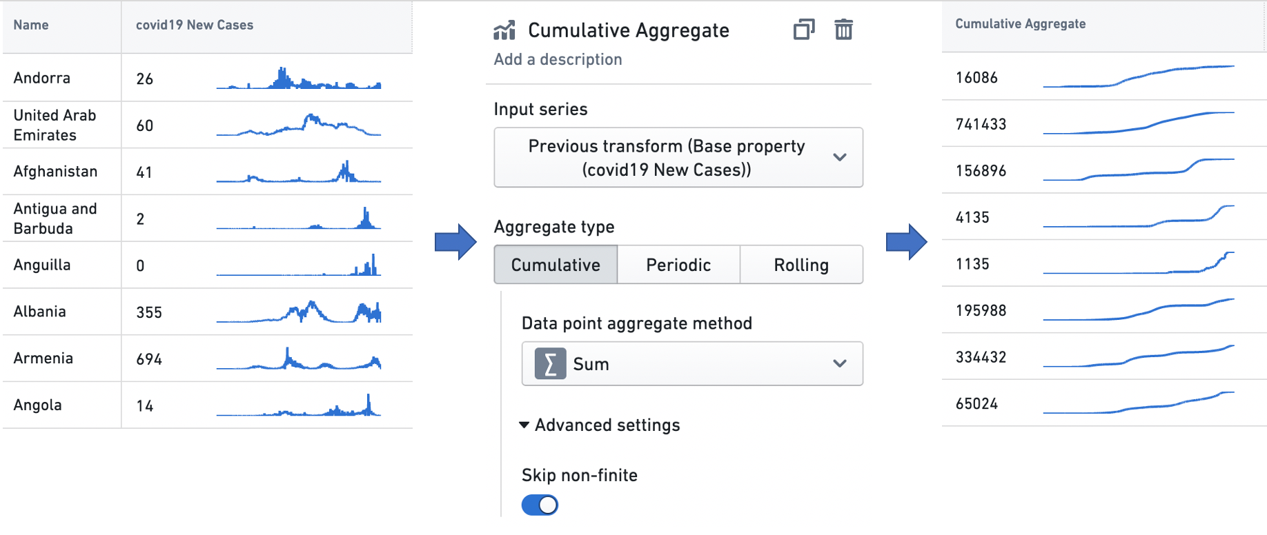
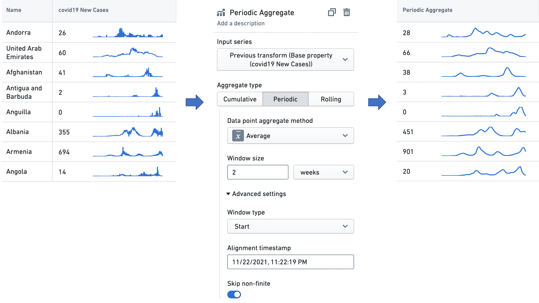
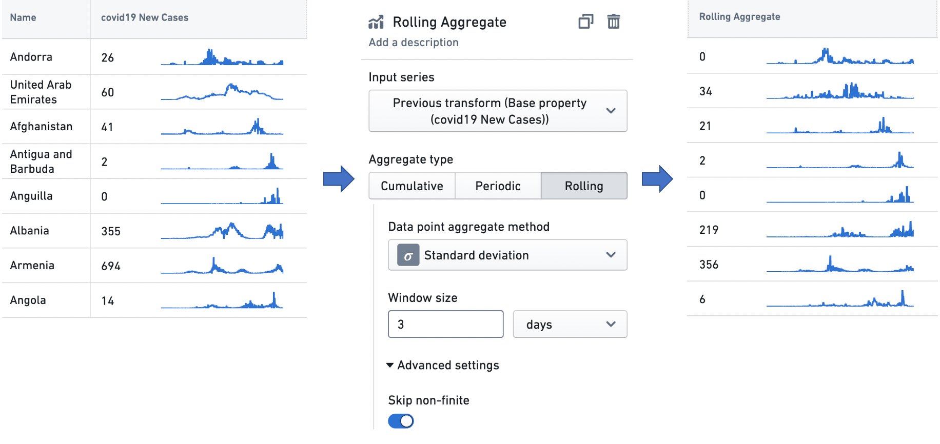
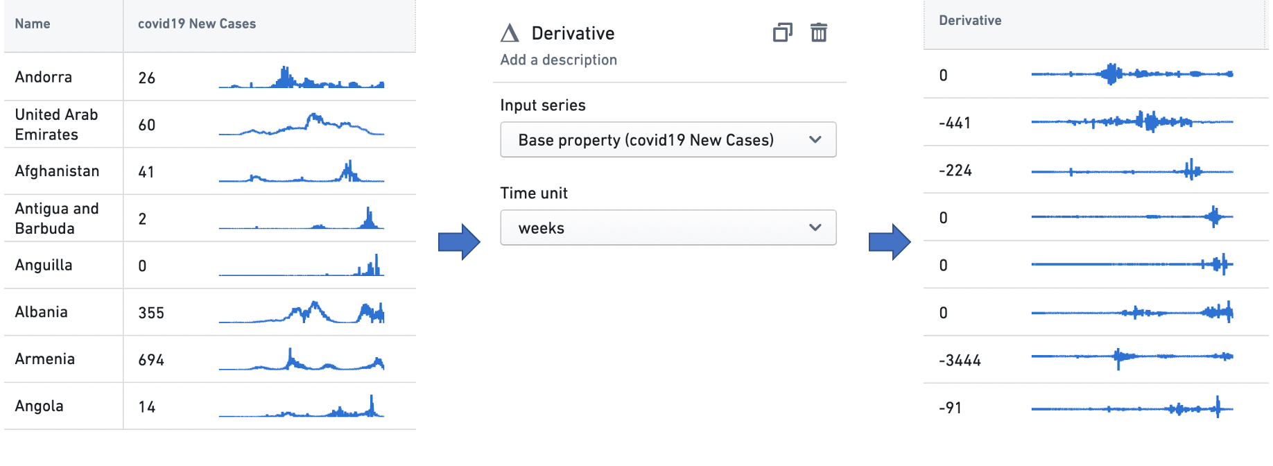
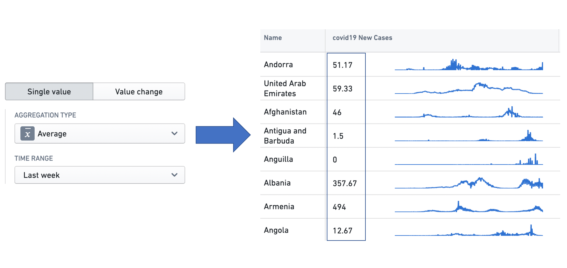
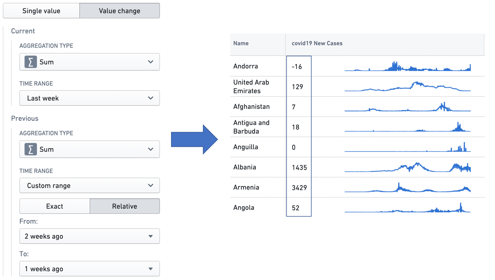
In the examples below, the Country object has a string property Name, which stores the name of the country, and a time series property covid19 New Cases, which stores a daily history of new COVID-19 cases observed in the country. This object is displayed in a Workshop Object table widget, and different time series transforms are applied to the covid19 New Cases time series property to generate new time series. The Object table widget is configured to display two visualizations for each time series: the latest value of the time series on the left, and a sparkline showing the history of the time series on the right.

Aggregate

The aggregate transform performs a windowed aggregation. Each point on the output time series is an aggregation on a group of points in the input time series. The aggregation method is user-specified — see the Time series summarizers section below for more information on the different aggregation types available.

There are three kinds of aggregate transform.

• Cumulative: Each output point is generated by taking a point on the input time series and aggregating over all earlier points, including the input point itself. For example, the configuration below creates a time series where each point represents the sum of the input values observed so far. The advanced settings allow the user to skip non-finite values in the input series when performing the operation.

• Periodic: Output points are generated at equally spaced, non-overlapping time intervals, and every output point is an aggregation over the input points that fall in its corresponding interval. These intervals are aligned with a user-specified alignment timestamp, and their length is defined by a user-specified window size. For example, the configuration below creates a time series of the average input values in the sequence of two week windows generated such that one of the windows — the alignment window — begins with the alignment timestamp. Along with skipping non-finite values in the input series, the advanced settings also allow the user to configure the following options:
• Window type: Start means that each output point represents the beginning of a time interval, and is an aggregate over the input points that follow it, while End means that each output point represents the end of a time interval, and is an aggregate over the input points that precede it.
• Alignment timestamp: Periodic intervals will be generated by starting at this timestamp, and offsetting by multiples of the window size.

• Rolling: Each output point is generated by taking a point on the input time series and aggregating over the points that fall in a fixed-size temporal window preceding it, including the input point itself. For example, the configuration below creates a time series where each point is the standard deviation of the input values observed in the three day window preceding it. The advanced settings allow the user to skip non-finite values in the input series when performing the operation.

Derivative

The derivative transform produces a time series representing the rate of change of the input time series. It also can perform a unit conversion on the rate of change, to enable interpretation with a user-specified time unit. For example, given a time series of the cumulative kilometer distance covered by a car over time, the transform can perform the scaling necessary to interpret the rate of change — the speed — at any point in terms of "kilometers/hour" (a common metric for measuring speed), "kilometers/second", or any similar temporal denominator.

In the example below, the derivative transform is configured to produce a weekly rate of change in COVID-19 case counts. These case observations are recorded daily, so there is one data point per day in the input time series, and a rate of change would ordinarily be interpreted as having the unit "cases/day". However, as the time unit for the transform is set to weeks, the transform scales the daily rates of change by a factor of seven (as there are seven days in a week), so the user can interpret the time series in the unit "cases/week".

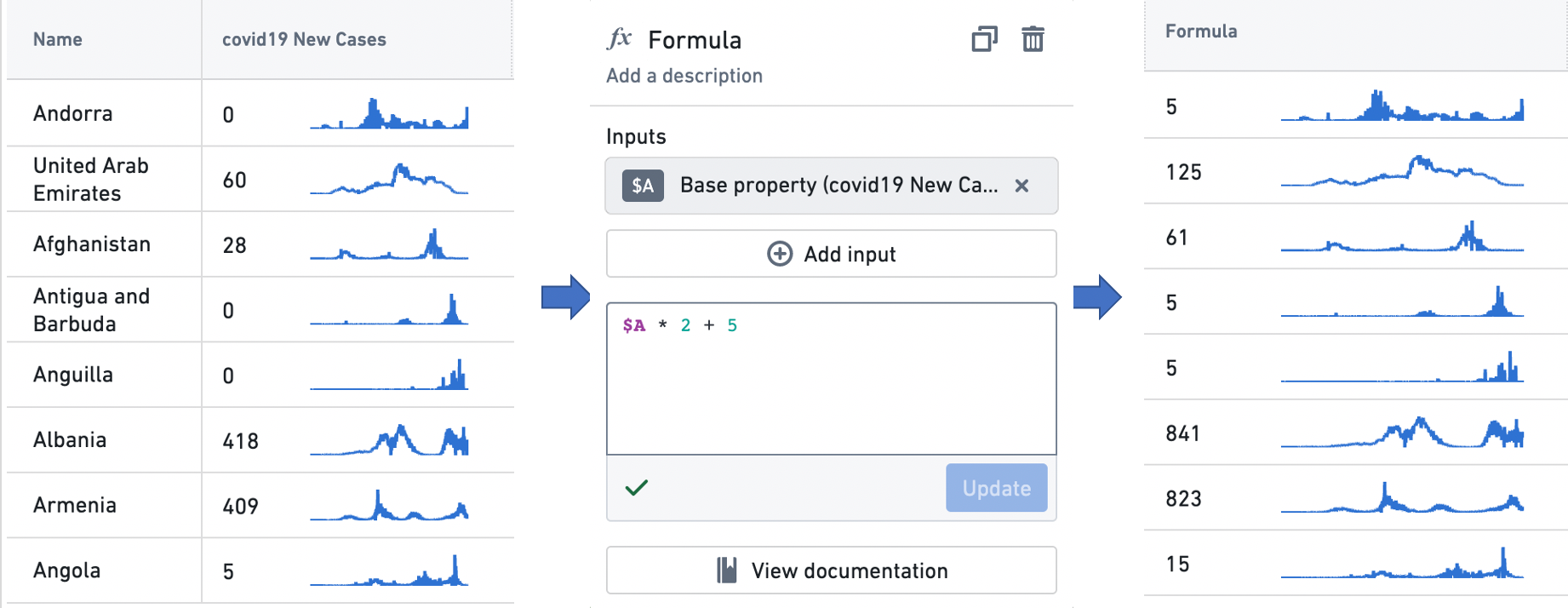
Formula

The formula transform computes a domain-specific language (DSL) formula on a set of input time series. Using the Add input button, users can add new input time series — either time series properties or the outputs from other transforms — to the transform, and then build formulas using variable references to these inputs. The example below scales the input time series by a factor of two, and adds five to the result.

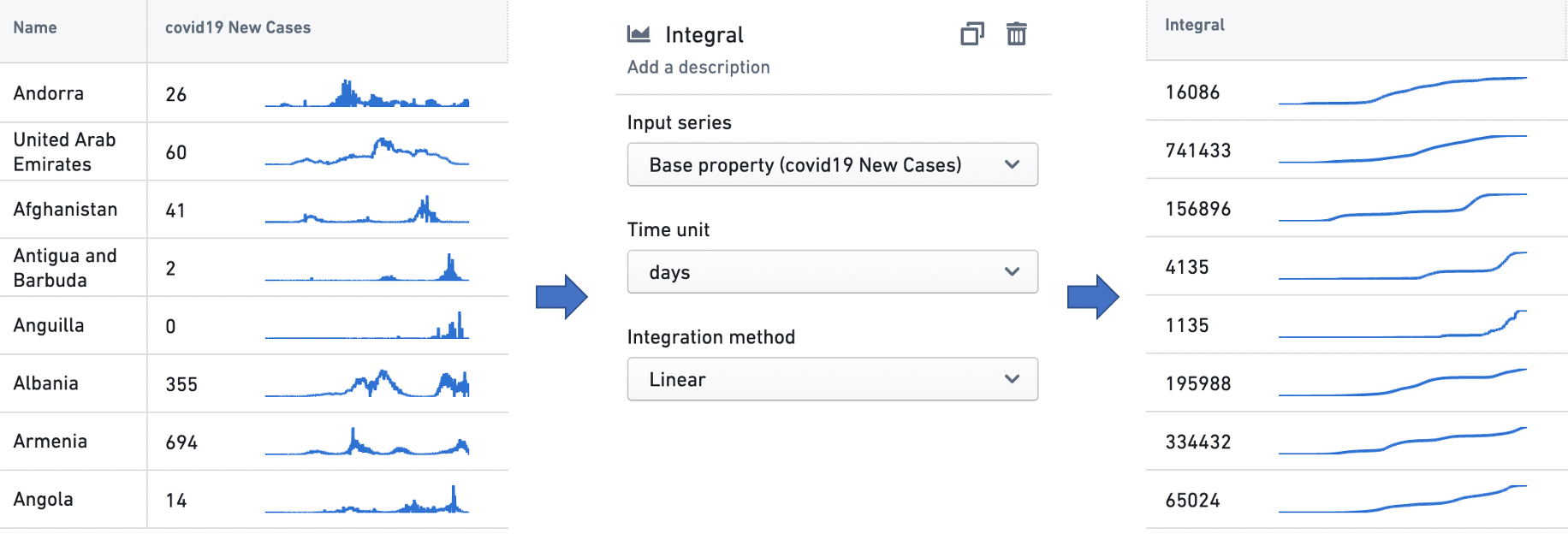
Integral

The integral transform produces a time series representing the cumulative area under the input time series when it is visualized as a graph. It also can perform a unit conversion on the area, to enable interpretation with a user-specified time unit. For example, given a time series of the kilowatt power consumption of a home, the transform can perform the scaling necessary to interpret the total area — the total energy consumed — at any point in terms of "kilowatt-hours" (the standard metric for measuring electricity consumption), "kilowatt-minutes", or any similar temporal numerator. The user can also specify the integration method, which is the method used to interpolate the value used between time series points. The options here are linear, which uses the average value between two time points; left hand sum, which uses the value at the earlier time point; and right hand sum, which uses the value at the later time point.

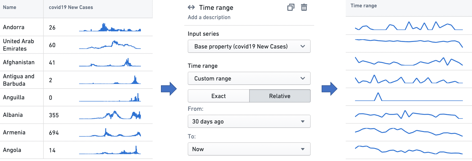
Time range

The time range transform filters an input time series to a user-specified time range. See the Time ranges section below for more information on specifying time ranges.

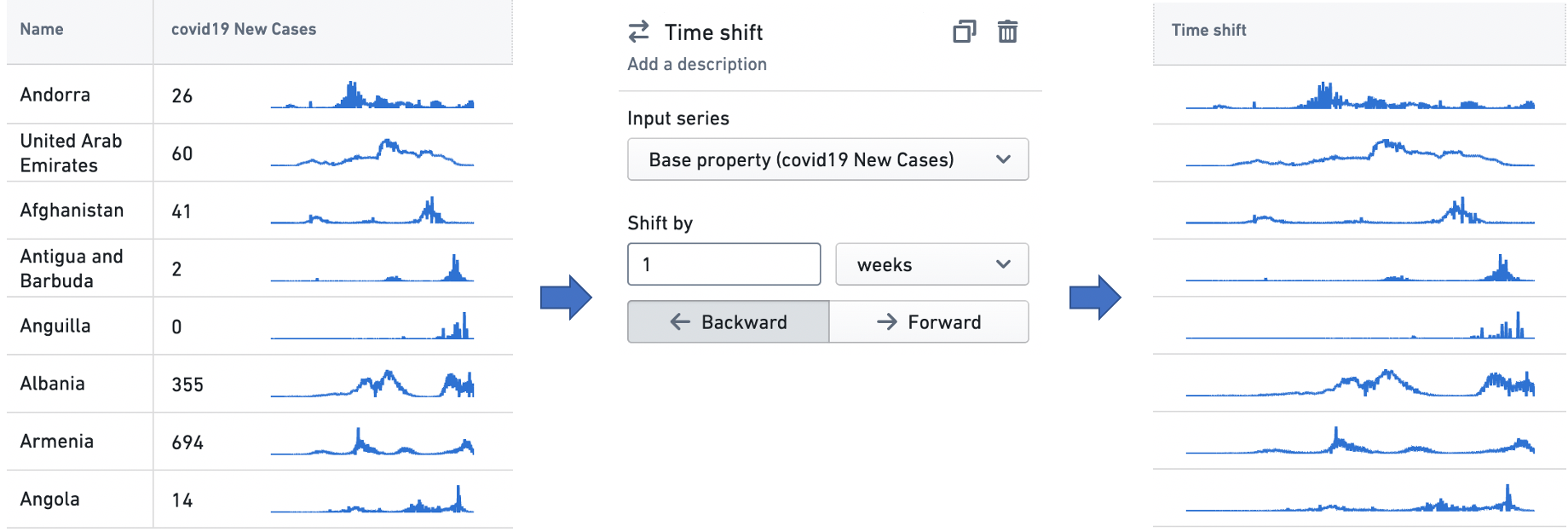
Time shift

The time shift transform generates an output time series that is identical to the input time series, but temporally shifted by a user-specified duration in a user-specified direction.

Time series summarizers

A time series summarizer configures a summary statistic for time series data; that is, a value that reflects the state of the time series. Summarizers are used in all Workshop widgets that support time series properties. For instance, the Object table and Metric card widgets use them to configure a single value to be displayed with a time series, as in the examples below. See Object table and Metric card for more information on the respective use cases.

There are two types of time series summarizer.

• Single Value: The Single Value summarizer computes and displays one aggregation for the time series input. For example, this Single value summarizer is set up to display the average number of COVID-19 cases from last week.

• Value Change: The Value Change summarizer computes two summarizers across the input data, and then calculates the difference between the two. This is especially useful in capturing changing trends. For example, this Value change summarizer computes the change in the weekly total number of COVID-19 cases observed between the last two weeks.

A summarizer is defined by an aggregation type, which specifies the calculation to be performed over the input data points, and a time range, which specifies the time range over which the aggregation is performed. See the Time ranges section below for more information on specifying time ranges.

The different aggregation types are as follows.

• Average: Calculates the mean over the input data points.
• Count: Gets the number of input data points in the time range.
• Difference: Calculates the difference between the values of the last point and the first point in the time range.
• First: Gets the value of the first data point in the time window.
• Last: Gets the value of the last data point in the time window.
• Min: Gets the minimum value among the data points in the time window.
• Max: Gets the maximum value among the data points in the time window.
• Product: Calculates the product of all the input values in the time range.
• Relative difference: Calculates the difference between the values of the last point and the first point in the time range, and divides this difference by the value of the first point. If multiplied by 100 (e.g. using a Formula transform), this produces the percentage change in the value of the time series over the time range.
• Standard deviation: Calculates the standard deviation of the input values in the time range.
• Sum: Calculates the sum over the input data points.

Time ranges

A time range specifies a finite interval of time, defined by its start and end times. We also call it a time window. Time ranges are used in time series transforms, to filter time series data using the time range transform; in time series summarizers, to specify the time window over which the aggregation is performed; and in the Object Table and Metric Card widgets, to configure sparklines and baselines. See Time series transforms, Time series summarizers, Object table and Metric card for more information on the respective use cases.

The interface to specify a time range is consistent across these applications. Users can select from one of the default options in the dropdown, or choose to specify a custom range.

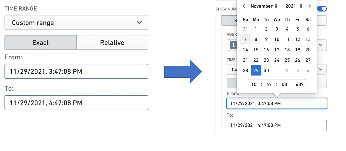
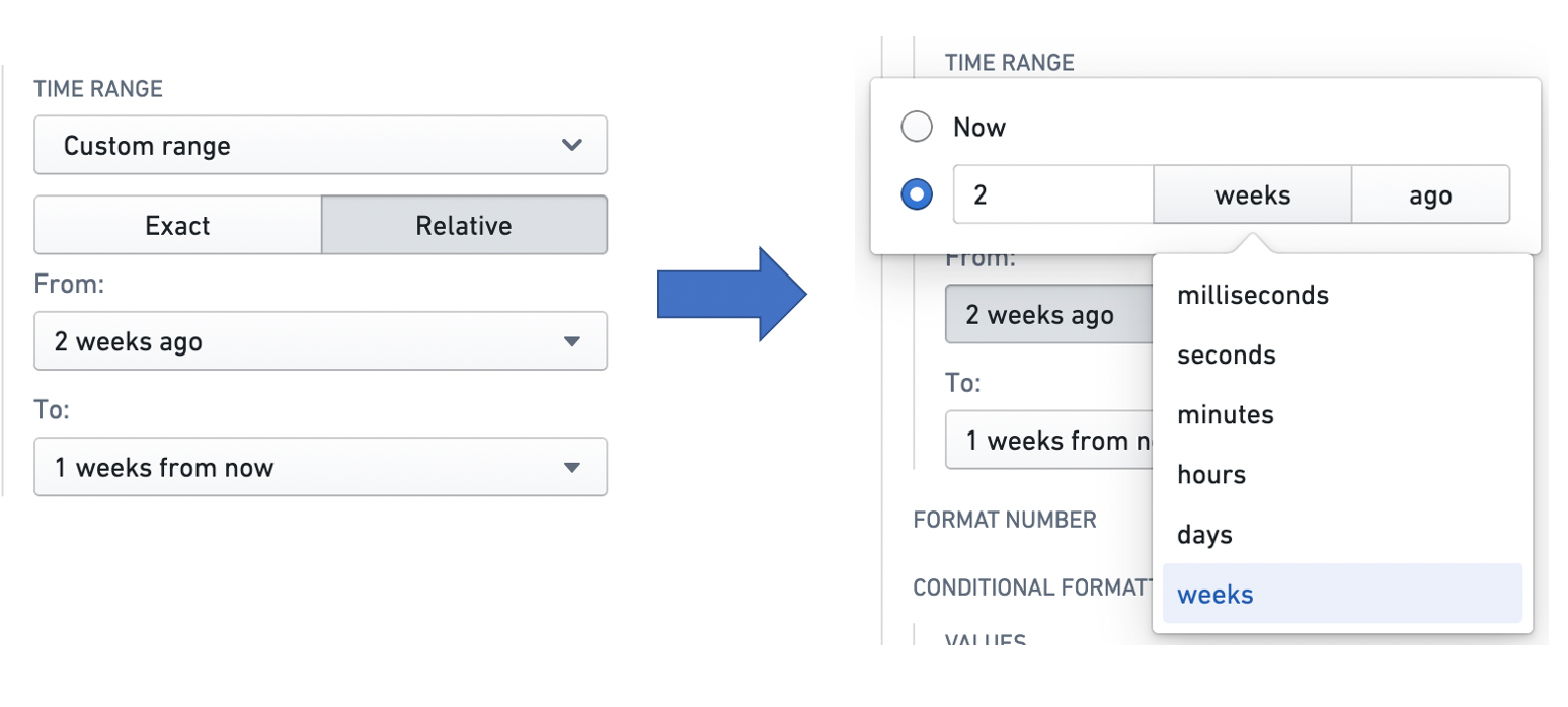
The custom range comes in two varieties: exact and relative.

The exact option uses a date and time picker to allow the user to specify absolute timestamps for the start and end of the range. The window specified here is absolute and hence does not change.

The relative option specifies the start and end of a window relative to the current time. Note that the current time is computed when it is first needed (e.g. when a user displays a widget using a relative time range). It then stays constant unless the web page is reloaded — this is to ensure consistency between widgets. Hence, the time window specified here is not an absolute window — it slides with the passing of time.

For example, a relative start of "2 weeks ago" specifies a window beginning December 1 when the application is opened on December 15, but December 2 when the application is opened on December 16. Similarly, a relative end of "1 week from now" specifies a window ending December 22 when the application is opened on December 15, but December 23 when it is opened on December 16. The window size can be specified in terms of milliseconds, seconds, minutes, hours, days, and weeks.

Baselines

A baseline is an additional time series line, rendered in combination with a sparkline in a visually distinguishing way (e.g. as a dotted line). By providing visual grounding and context for a time series, a baseline can help users interpret trends. Baselines can be configured in the Object Table and Metric Card widgets.

There are three types of baseline: Static, Numeric property, and Time series property.

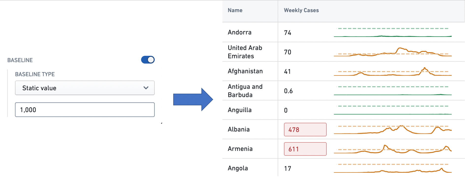
The Static type means that the value of the baseline for every time series is a static user-specified value. The user can input this value into a text box. In this example, the Weekly Cases column has a baseline with a static value of 1000.

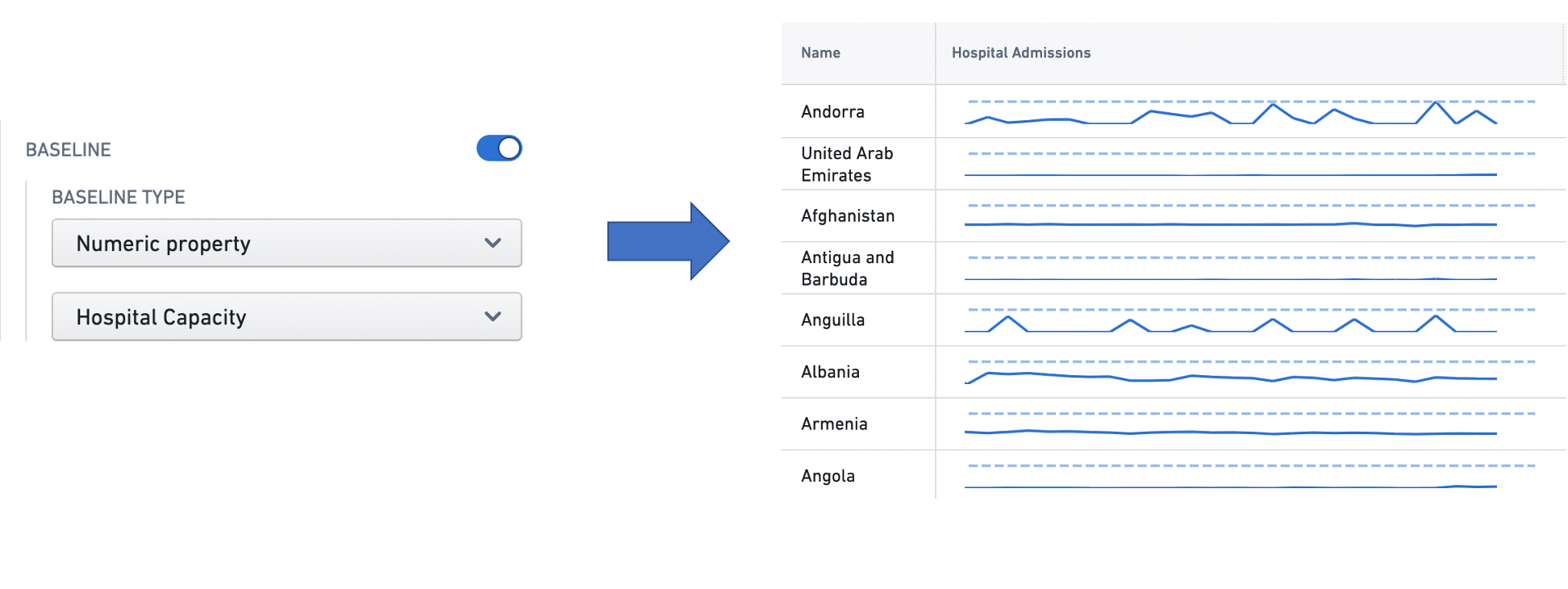
The Numeric property type means that the user can specify a numeric property of the object type feeding the widget, whose value for each object is used as the baseline for the corresponding series. See Property for more information on object properties. In this example, each row in the Hospital Admissions column has a baseline whose value is the value of the Hospital Capacity property of the corresponding Country object.

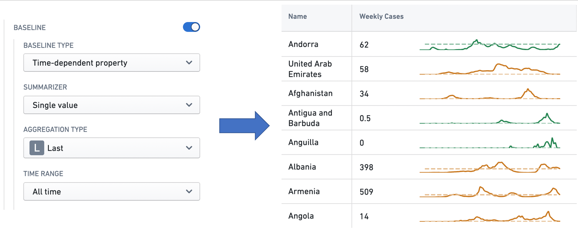
The Time series type means that the user can configure a time series summarizer to generate a unique baseline value for every series. See Time series properties in Workshop for more information on summarizers. In this example, each time series in the Weekly Cases column has a baseline with the value of the most recent observation in the time series.

---

中文翻译

---

时间序列属性(Time series properties)

:::callout 时间序列属性需要先安装时间序列服务(Time series services)，因此您的Foundry实例可能暂不支持该功能。如有疑问，请联系您的Palantir客户代表。 :::

时间序列属性(time series property) 是一种特殊的对象属性类型。常规对象属性仅存储单个值（例如字符串Argentina或数字81231），而时间序列属性存储带时间戳的历史值序列。您可以查阅创建时间序列属性了解更多相关信息。

在Workshop中，时间序列属性（包括通过时间序列转换(time series transforms)生成的时间序列）可以通过创建时间序列集(time series set) 变量，或直接访问目标对象的对应属性，在XY图表(Chart XY)、地图(Map)、指标卡片(Metric Card)和对象表格(Object Table)组件中使用。如需了解时间序列属性的使用方法，请参考对应功能的文档：

• XY图表
• 地图
• 指标卡片
• 对象表格
• 变量

时间序列转换(Time series transforms)

时间序列转换(time series transform) 会对输入的时间序列数据执行数学运算，生成新的输出时间序列。输入的时间序列可以是时间序列属性，也可以是其他转换的输出，因此支持多个转换链式调用。

在下方示例中，Country对象有一个字符串属性Name（存储国家名称）和一个时间序列属性covid19 New Cases（存储该国每日新增COVID-19病例的历史数据）。该对象展示在Workshop的对象表格组件中，我们对covid19 New Cases时间序列属性应用不同的时间序列转换来生成新的时间序列。对象表格组件配置为每个时间序列展示两种可视化效果：左侧展示时间序列的最新值，右侧展示反映数值历史走势的迷你图(sparkline)。

聚合(Aggregate)

聚合转换会执行窗口聚合运算。输出时间序列的每个点都是对输入时间序列中一组点的聚合结果。聚合方法由用户指定，您可以查阅下方时间序列汇总器(Time series summarizers)部分了解可用的聚合类型详情。

共有三种聚合转换：

• 累计(Cumulative)： 每个输出点由输入时间序列的对应点及其之前的所有点聚合生成。例如下方配置生成的时间序列中，每个点代表到该时间点为止输入值的总和。高级设置支持用户在执行运算时跳过输入序列中的非有限值。

• 周期(Periodic)： 输出点按等间隔、无重叠的时间区间生成，每个输出点是对应时间区间内输入点的聚合结果。这些区间与用户指定的对齐时间戳对齐，区间长度由用户指定的窗口大小定义。例如下方配置生成的时间序列，每个点是每两周窗口内输入值的平均值，其中一个窗口（对齐窗口）的起始时间就是指定的对齐时间戳。 除了支持跳过输入序列中的非有限值外，高级设置还支持用户配置以下选项：
• 窗口类型：Start表示每个输出点对应时间区间的起始位置，聚合的是该点之后的输入点；End表示每个输出点对应时间区间的结束位置，聚合的是该点之前的输入点。
• 对齐时间戳：周期区间将从该时间戳开始，按窗口大小的倍数偏移生成。

• 滚动(Rolling)： 每个输出点由输入时间序列的对应点及其之前固定大小时间窗口内的所有点聚合生成。例如下方配置生成的时间序列中，每个点是该时间点之前三天窗口内输入值的标准差。高级设置支持用户在执行运算时跳过输入序列中的非有限值。

导数(Derivative)

导数转换生成的时间序列代表输入时间序列的变化率。它还支持对变化率进行单位转换，方便用户按指定的时间单位解读结果。例如，给定一辆汽车累计行驶公里数的时间序列，该转换可以做相应缩放，让用户可以按“公里/小时”（常用的速度单位）、“公里/秒”或其他类似时间分母的单位解读任意时间点的变化率（即速度）。

在下方示例中，导数转换被配置为输出COVID-19病例数的周变化率。病例数据按日记录，因此输入时间序列每天有一个数据点，默认的变化率单位是“例/天”。但由于转换的时间单位设置为weeks，转换会将日变化率乘以7（一周有7天），用户就可以按“例/周”的单位解读该时间序列。

公式(Formula)

公式转换基于领域特定语言(DSL, domain-specific language)对一组输入时间序列执行公式计算。用户可以通过Add input按钮添加新的输入时间序列（可以是时间序列属性，也可以是其他转换的输出），然后通过引用这些输入的变量构建公式。下方示例将输入时间序列的数值乘以2，再加上5。

积分(Integral)

积分转换生成的时间序列代表输入时间序列可视化成曲线后的累计面积。它还支持对面积进行单位转换，方便用户按指定的时间单位解读结果。例如，给定一个家庭的千瓦级功耗时间序列，该转换可以做相应缩放，让用户可以按“千瓦时”（标准的用电量单位）、“千瓦·分钟”或其他类似时间分子的单位解读任意时间点的总面积（即总耗电量）。用户还可以指定积分方法，即时间序列点之间的插值方法，可选值包括：linear（线性，取两个时间点之间的平均值）、left hand sum（左和，取更早时间点的值）、right hand sum（右和，取更晚时间点的值）。

时间范围(Time range)

时间范围转换会将输入时间序列过滤到用户指定的时间区间内。如需了解指定时间范围的更多信息，请查阅下方时间范围(Time ranges)部分。

时间偏移(Time shift)

时间偏移转换生成的输出时间序列与输入时间序列完全一致，只是按用户指定的方向和时长做了整体时间偏移。

时间序列汇总器(Time series summarizers)

时间序列汇总器(time series summarizer) 用于配置时间序列数据的汇总统计量，也就是反映时间序列状态的单个值。所有支持时间序列属性的Workshop组件都可以使用汇总器。例如，对象表格和指标卡片组件使用汇总器配置时间序列对应的展示值，如下方示例所示。您可以查阅对象表格和指标卡片了解各自的使用场景。

共有两类时间序列汇总器：

• 单值(Single Value)： 单值汇总器对输入时间序列计算并展示一个聚合值。例如，这个单值汇总器被配置为展示上周COVID-19的平均新增病例数。

• 值变化(Value Change)： 值变化汇总器对输入数据计算两个汇总值，然后得出两者的差值。这对于捕捉变化趋势尤其有用。例如，这个值变化汇总器计算过去两周观察到的COVID-19周累计病例数的变化。

汇总器由聚合类型(aggregation type) 和时间范围(time range) 两个部分定义：聚合类型指定对输入数据点执行的计算逻辑，时间范围指定执行聚合的时间窗口。如需了解指定时间范围的更多信息，请查阅下方时间范围(Time ranges)部分。

可用的聚合类型如下：

• 平均值(Average)： 计算输入数据点的均值。
• 计数(Count)： 统计时间范围内输入数据点的数量。
• 差值(Difference)： 计算时间范围内最后一个点和第一个点的数值差。
• 首个值(First)： 取时间窗口内第一个数据点的数值。
• 最新值(Last)： 取时间窗口内最后一个数据点的数值。
• 最小值(Min)： 取时间窗口内数据点的最小值。
• 最大值(Max)： 取时间窗口内数据点的最大值。
• 乘积(Product)： 计算时间范围内所有输入值的乘积。
• 相对差值(Relative difference)： 计算时间范围内最后一个点和第一个点的数值差，再除以第一个点的数值。如果乘以100（例如使用公式转换），就可以得到时间序列在该时间范围内的变化百分比。
• 标准差(Standard deviation)： 计算时间范围内输入值的标准差。
• 总和(Sum)： 计算输入数据点的总和。

时间范围(Time ranges)

时间范围(time range) 指定一个有限的时间区间，由起始时间和结束时间定义，也称为时间窗口(time window)。时间范围的应用场景包括：在时间序列转换中，通过时间范围转换过滤时间序列数据；在时间序列汇总器中，指定执行聚合的时间窗口；在对象表格和指标卡片组件中，配置迷你图和基线(baseline)。您可以查阅时间序列转换、时间序列汇总器、对象表格和指标卡片了解各自的使用场景。

上述所有应用场景中指定时间范围的界面都是一致的。用户可以从下拉菜单的默认选项中选择，也可以选择自定义范围。

自定义范围分为两种：精确和相对。

精确选项使用日期时间选择器，允许用户指定范围起止的绝对时间戳。此处指定的窗口是固定的，不会发生变化。

相对选项指定相对于当前时间的窗口起止时间。请注意，当前时间会在首次需要时计算（例如用户打开使用相对时间范围的组件时），之后会保持不变，除非网页重新加载——这是为了保证不同组件之间的一致性。因此，此处指定的时间窗口不是绝对的，会随时间推移自动滑动。

例如：当用户12月15日打开应用时，“2周前”的相对起始时间代表窗口从12月1日开始；如果12月16日打开应用，窗口就从12月2日开始。同理，“1周后”的相对结束时间在12月15日打开应用时代表窗口到12月22日结束，12月16日打开则到12月23日结束。窗口大小支持的单位包括毫秒、秒、分钟、小时、天和周。

基线(Baselines)

基线(baseline) 是额外的时间序列线，会以视觉上有区分度的样式（例如虚线）和迷你图一同渲染。基线可以为时间序列提供视觉参照和上下文，帮助用户解读趋势。用户可以在对象表格和指标卡片组件中配置基线。

共有三种基线类型：Static（静态）、Numeric property（数值属性）和Time series property（时间序列属性）。

Static类型指所有时间序列的基线值都是用户指定的静态值，用户可以在文本框中输入该值。在本示例中，Weekly Cases列的基线静态值为1000。

Numeric property类型指用户可以指定为组件提供数据的对象类型的某个数值属性，每个对象的该属性值会作为对应时间序列的基线。如需了解对象属性的更多信息，请查阅属性。在本示例中，Hospital Admissions列每一行的基线值是对应Country对象的Hospital Capacity属性值。

Time series类型指用户可以配置时间序列汇总器为每个序列生成唯一的基线值。如需了解汇总器的更多信息，请查阅Workshop中的时间序列属性。在本示例中，Weekly Cases列每个时间序列的基线值是该时间序列的最新观测值。