Time Series Analysis（时间序列分析(Time Series Analysis)）

The Time Series Analysis widget enables users to independently investigate time series data with flexibility, within the framework of the Workshop application.

Available plots

Add time series data from the Ontology with the + Add Data search bar, then derive new plots by selecting New Plot. Plots can be organized across multiple canvases within the same analysis.

Time series plots

• Bollinger bands: Plot upper and lower bands at a configurable number of standard deviations around a moving average.
• Combine time series: Merge multiple time series into a single plot, specifying how to handle overlapping time points (for example, mean, min, or max).
• Cumulative aggregate: Display the cumulative value of a series over the entire length of the series or over a specific period of time.
• Derivative: Display the rate of change at each point in the selected input series.
• DSP filter: Apply a digital signal processing filter (Butterworth, Chebyshev, or inverse Chebyshev) to reduce noise in a time series.
• Event statistics: Aggregate a time series over intervals where an event occurs, returning one point per event.
• Filter time series: Keep or remove points in a time series based on a time range or mathematical condition.
• Formula time series: Create a new plot by applying a mathematical formula across one or more time series using Quiver's formula language.
• Integral: Calculate the area under the curve of a time series, the inverse of a derivative.
• Linear aggregation: Compute a linear aggregation across multiple time series over time.
• Periodic aggregate: Downsample a time series by aggregating data over fixed time periods, producing one point per period.
• Rolling aggregate: Calculate a new point for each data point based on a rolling window function and aggregate method, typically used to smooth a series.
• Sample: Resample a time series at a constant frequency to fill gaps or change the data rate.
• Shift time series: Shift the time of a series forwards or backwards by a specified duration.

Event sets

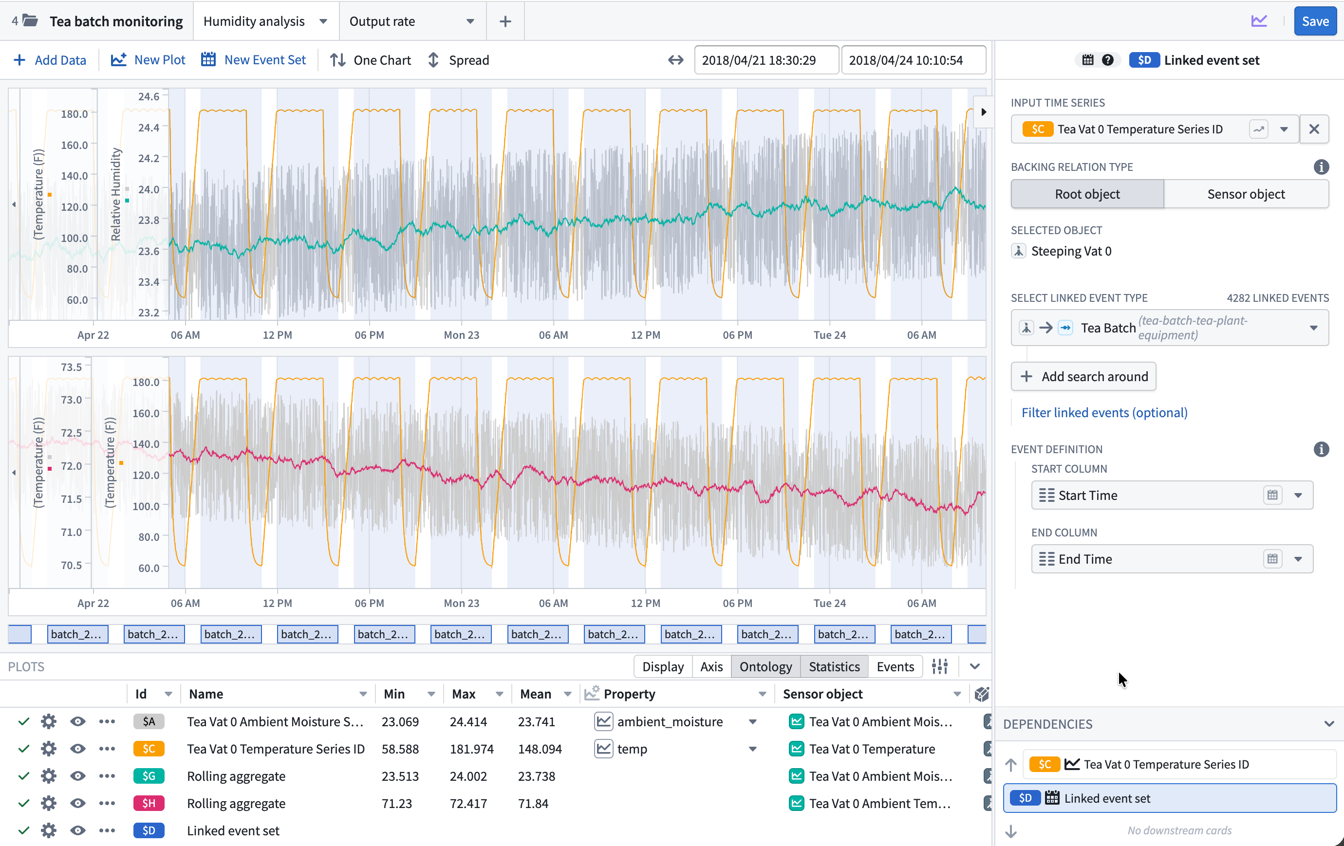
• Linked event set: Create an event set from linked objects in the Ontology by traversing object relationships and specifying which properties hold the start and end timestamps.
• Time series search: Create an event set from conditions on time series data, identifying time ranges that match a specified pattern or threshold.

Visualization options

The Plots panel at the bottom of the widget contains settings and information that are common to all plot types. Data configurations specific to the plot type are controlled in the editor panel on the right side of the widget. Column visibility, ordering, sorting, and widths are all customizable. Use the Configure columns menu for fine-grained control of the column ordering and to add non-default columns.

The following visualization options can be quickly toggled from the panel header:

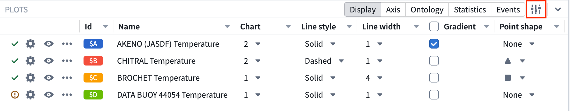
Display

• Chart: The canvas chart that the plot is rendered on.
• Line style: Render the plot line as solid or dashed.
• Line width: The thickness of the plot line.
• Gradient: Toggle gradient shading under the plot line.
• Point shape: The shape of data points (circle, triangle, square, diamond, or none).
• Point size: The size of data points. Disabled when point shape is set to none.

Axis

• Axis: The Y-axis assignment for the plot. Select from existing axes with a compatible unit, or create a new axis.
• Unit: The unit of the Y-axis. Allows unit conversion (for example, meters to kilometers) or custom label overrides.
• Auto scale: Toggle automatic axis scaling to fit the data extent.
• Axis min: The minimum value of the Y-axis range. Disabled when auto scale is active.
• Axis max: The maximum value of the Y-axis range. Disabled when auto scale is active.

Ontology

• Root object: The Ontology object that the time series property is located on, or the root object if the time series is a sensor. Selecting a different object updates the plot and any dependent derived plots. When all plots have the same root object, this column can be bulk updated using the button in the column header.
• Sensor object: The sensor object associated with the time series (if applicable).
• Property: The time series property or sensor name. Selecting a different property updates the plot and any dependent derived plots. When all plots are using the same property, this column can be bulk updated using the button in the column header.

Statistics

• Min: The minimum value of the plot within the current view range.
• Max: The maximum value of the plot within the current view range.
• Mean: The mean value of the plot within the current view range.

Events

• Event count: The number of events within the current view range for event set plots.
• Event highlight: Toggle chart highlighting for time ranges where events occur.

Additional configurations can be added from the Column configuration menu:

Axis display options

• Align axis: Align the axis to the left or right side of the chart.
• Log scale: Display the axis using a logarithmic scale.
• Invert axis: Invert the direction of the axis.

Point display options

• Point fill: The fill color of data points. Disabled when point shape is set to none.
• Point outline width: The outline width of data points. Disabled when point fill is set to none or is the same as the plot color.

Interpolation

• Internal interpolation: The interpolation method used to connect data points within the time series.
• External interpolation: The interpolation method used before the first data point and after the last data point.

Learn more about available interpolation options.

Configuration options

Add data options

• Enable users to select time series data from the Ontology, optionally restricting which object types are available. To further narrow the available series, apply object set filters for each object type.
• Control series with object sets: Initialize the analysis with a controlled set of time series by specifying object sets and time series properties. Users cannot delete or edit the data configuration for these series but can customize the display from the Plot Details panel.
• Add initial event sets: Initialize the analysis with event sets backed by object sets, specifying the properties to use for event start and end times. Users cannot delete or edit the data configuration for these series but can customize the display from the Plot Details panel.

Plot options

• New plot placement: Choose which canvas new plots are added to by default.
• Customize available plot types: Control which derived plot types are available from the New plot menu and the order in which they appear.
• Customize available event set types: Control which types of event sets can be added by the user.

Chart options

• Overlay Y-axes: When enabled, Y-axes are rendered as transparent overlays. Otherwise, the Y-axes will shift the chart data to the side.
• Collapse Y-axes by default: Start with Y-axes collapsed to save chart space.
• Display Y-axes boundaries when collapsed: Display axis boundaries when axes are collapsed.
• Tooltip options: Configure tooltip visibility, displayed values, time and label formatting, text wrapping, and the number of significant digits.
• Enable UTC time format: Display chart time values in UTC format.
• Sync X-axes across canvases: Keep the X-axis view range synchronized when zooming or panning across multiple canvases.
• Default view range: The initial view range for time series charts in the analysis. The available options include:
• Full data range: Use the start and end dates of the included time series. Note that this may negatively impact performance for large time series.
• Fixed date range: Use workshop variables to define absolute start and end dates.
• Relative date range: Use workshop variables to define a range relative to the time when the page was loaded (for example, "2 weeks ago to now").

Resource options

• Enable analysis saving: Save and share analyses for future reference. Analyses can be saved as either Private or Public.
• Configure default save location: Select a folder or use a string variable to provide the default save location.
• Don't allow users to choose save location: Always use the default save location and hide the save location select in the UI.
• Output analysis RID: Store the resource identifier of the active analysis in a string variable for use elsewhere in the Workshop application.
• Autoload analyses: Specify analyses to load automatically when the widget initializes. Display options from the widget configuration (for example, tooltip options) will override those saved on the analysis, but the analysis will retain its original settings when saved from the widget.
• Don't clear on load: When disabled, updating the autoloaded analysis RIDs will reset the widget view state. If enabled, updating the analysis RIDs will add new analyses to the view state, but will not clear analyses currently being viewed.

Save an analysis for later use

• Save as a time series analysis resource: Toggle on the Enable analysis saving configuration to allow users to preserve and easily share their analyses. Saved analyses can be opened in a standalone resource view or loaded into the Workshop widget using its RID.
• Open in Quiver: Select Open in Quiver from the upper right corner of the widget header to transfer the analysis to a full Quiver analysis for more advanced time series workflows. This creates a new Quiver analysis with the same canvases and plots. Note that changes made in the Quiver analysis are not reflected back in the Workshop widget.

---

中文翻译

---

时间序列分析(Time Series Analysis)

时间序列分析(Time Series Analysis) 组件使用户能够在 Workshop 应用框架内，灵活地独立研究时间序列数据。

可用图表(Plots)

通过 + 添加数据(Add Data) 搜索栏从本体论(Ontology)添加时间序列数据，然后选择 新建图表(New Plot) 来派生新图表。图表可以在同一分析中的多个画布(Canvases)上组织排列。

时间序列图表(Time series plots)

• 布林带(Bollinger bands): 在移动平均线周围绘制可配置标准差倍数的上轨和下轨。
• 合并时间序列(Combine time series): 将多个时间序列合并到单个图表中，并指定如何处理重叠的时间点（例如，平均值、最小值或最大值）。
• 累计聚合(Cumulative aggregate): 显示序列在整个长度或特定时间段内的累计值。
• 导数(Derivative): 显示所选输入序列中每个点的变化率。
• DSP 滤波器(DSP filter): 应用数字信号处理滤波器（巴特沃斯、切比雪夫或逆切比雪夫）以减少时间序列中的噪声。
• 事件统计(Event statistics): 在事件发生的间隔内聚合时间序列，每个事件返回一个数据点。
• 过滤时间序列(Filter time series): 基于时间范围或数学条件，保留或移除时间序列中的数据点。
• 公式时间序列(Formula time series): 使用 Quiver 的公式语言，通过在一个或多个时间序列上应用数学公式来创建新图表。
• 积分(Integral): 计算时间序列曲线下的面积，是导数的逆运算。
• 线性聚合(Linear aggregation): 随时间对多个时间序列执行线性聚合。
• 周期聚合(Periodic aggregate): 通过在固定时间段内聚合数据来对时间序列进行降采样，每个周期生成一个数据点。
• 滚动聚合(Rolling aggregate): 基于滚动窗口函数和聚合方法，为每个数据点计算新值，通常用于平滑序列。
• 重采样(Sample): 以恒定频率对时间序列进行重采样，以填补数据空缺或改变数据速率。
• 时间平移(Shift time series): 将序列的时间向前或向后移动指定的时长。

事件集(Event sets)

• 关联事件集(Linked event set): 通过遍历对象关系并指定哪些属性包含开始和结束时间戳，从本体论(Ontology)中的关联对象创建事件集。
• 时间序列搜索(Time series search): 根据时间序列数据的条件创建事件集，识别符合指定模式或阈值的时间范围。

可视化选项(Visualization options)

组件底部的 图表(Plots) 面板包含所有图表类型通用的设置和信息。特定于图表类型的数据配置在组件右侧的编辑面板中进行控制。列的可见性、顺序、排序和宽度均可自定义。使用 配置列(Configure columns) 菜单可以精细控制列的顺序并添加非默认列。

以下可视化选项可以从面板标题快速切换：

显示(Display)

• 图表(Chart): 渲染图表的画布(Canvas chart)。
• 线条样式(Line style): 将图表线条渲染为实线或虚线。
• 线条宽度(Line width): 图表线条的粗细。
• 渐变(Gradient): 切换图表线条下方的渐变阴影。
• 点形状(Point shape): 数据点的形状（圆形、三角形、正方形、菱形或无）。
• 点大小(Point size): 数据点的大小。当点形状设置为无时禁用。

坐标轴(Axis)

• 坐标轴(Axis): 图表的 Y 轴分配。从具有兼容单位的现有坐标轴中选择，或创建新坐标轴。
• 单位(Unit): Y 轴的单位。允许单位转换（例如，米到千米）或自定义标签覆盖。
• 自动缩放(Auto scale): 切换自动缩放坐标轴以适应数据范围。
• 坐标轴最小值(Axis min): Y 轴范围的最小值。当自动缩放激活时禁用。
• 坐标轴最大值(Axis max): Y 轴范围的最大值。当自动缩放激活时禁用。

本体论(Ontology)

• 根对象(Root object): 时间序列属性所在的本体论(Ontology)对象，或者如果时间序列是传感器(sensor)，则为根对象。选择不同的对象会更新图表及其任何依赖的派生图表。当所有图表具有相同的根对象时，可以使用列标题中的按钮批量更新此列。
• 传感器对象(Sensor object): 与时间序列关联的传感器对象（如果适用）。
• 属性(Property): 时间序列属性或传感器名称。选择不同的属性会更新图表及其任何依赖的派生图表。当所有图表使用相同的属性时，可以使用列标题中的按钮批量更新此列。

统计信息(Statistics)

• 最小值(Min): 当前视图范围内图表的最小值。
• 最大值(Max): 当前视图范围内图表的最大值。
• 平均值(Mean): 当前视图范围内图表的平均值。

事件(Events)

• 事件计数(Event count): 对于事件集图表，当前视图范围内的事件数量。
• 事件高亮(Event highlight): 切换事件发生时间范围的图表高亮显示。

可以从 列配置(Column configuration) 菜单添加其他配置：

坐标轴显示选项(Axis display options)

• 对齐坐标轴(Align axis): 将坐标轴对齐到图表的左侧或右侧。
• 对数刻度(Log scale): 使用对数刻度显示坐标轴。
• 反转坐标轴(Invert axis): 反转坐标轴的方向。

点显示选项(Point display options)

• 点填充(Point fill): 数据点的填充颜色。当点形状设置为无时禁用。
• 点轮廓宽度(Point outline width): 数据点的轮廓宽度。当点填充设置为无或与图表颜色相同时禁用。

插值(Interpolation)

• 内部插值(Internal interpolation): 用于连接时间序列内数据点的插值方法。
• 外部插值(External interpolation): 在第一个数据点之前和最后一个数据点之后使用的插值方法。

了解有关可用插值选项的更多信息。

配置选项(Configuration options)

添加数据选项(Add data options)

• 允许用户选择时间序列数据 来自本体论(Ontology)，并可选择限制可用的对象类型。要进一步缩小可用序列范围，请为每种对象类型应用对象集过滤器。
• 使用对象集控制序列(Control series with object sets): 通过指定对象集和时间序列属性，使用受控的时间序列集初始化分析。用户无法删除或编辑这些序列的数据配置，但可以从 图表详情(Plot Details) 面板自定义显示。
• 添加初始事件集(Add initial event sets): 使用由对象集支持的事件集初始化分析，指定用于事件开始和结束时间的属性。用户无法删除或编辑这些序列的数据配置，但可以从 图表详情(Plot Details) 面板自定义显示。

图表选项(Plot options)

• 新图表放置位置(New plot placement): 选择默认将新图表添加到哪个画布(Canvas)。
• 自定义可用图表类型(Customize available plot types): 控制 新建图表(New plot) 菜单中可用的派生图表类型及其显示顺序。
• 自定义可用事件集类型(Customize available event set types): 控制用户可以添加的事件集类型。

图表选项(Chart options)

• 叠加 Y 轴(Overlay Y-axes): 启用后，Y 轴将渲染为透明叠加层。否则，Y 轴会将图表数据向一侧偏移。
• 默认折叠 Y 轴(Collapse Y-axes by default): 启动时折叠 Y 轴以节省图表空间。
• 折叠时显示 Y 轴边界(Display Y-axes boundaries when collapsed): 当坐标轴折叠时显示坐标轴边界。
• 工具提示选项(Tooltip options): 配置工具提示的可见性、显示的值、时间和标签格式、文本换行以及有效数字位数。
• 启用 UTC 时间格式(Enable UTC time format): 以 UTC 格式显示图表时间值。
• 跨画布同步 X 轴(Sync X-axes across canvases): 在多个画布(Canvases)上缩放或平移时，保持 X 轴视图范围同步。
• 默认视图范围(Default view range): 分析中时间序列图表的初始视图范围。可用选项包括：
• 完整数据范围(Full data range): 使用包含的时间序列的开始和结束日期。请注意，对于大型时间序列，这可能会对性能产生负面影响。
• 固定日期范围(Fixed date range): 使用 Workshop 变量定义绝对的开始和结束日期。
• 相对日期范围(Relative date range): 使用 Workshop 变量定义相对于页面加载时间的范围（例如，"2周前到现在"）。

资源选项(Resource options)

• 启用分析保存(Enable analysis saving): 保存和共享分析以供将来参考。分析可以保存为 私有(Private) 或 公开(Public)。
• 配置默认保存位置(Configure default save location): 选择一个文件夹或使用字符串变量提供默认保存位置。
• 不允许用户选择保存位置(Don't allow users to choose save location): 始终使用默认保存位置，并在 UI 中隐藏保存位置选择器。
• 输出分析 RID(Output analysis RID): 将活动分析的资源标识符存储在字符串变量中，以便在 Workshop 应用的其他地方使用。
• 自动加载分析(Autoload analyses): 指定组件初始化时自动加载的分析。来自组件配置的显示选项（例如，工具提示选项）将覆盖保存在分析上的设置，但从组件保存分析时，分析将保留其原始设置。
• 加载时不清除(Don't clear on load): 禁用时，更新自动加载的分析 RID 将重置组件视图状态。如果启用，更新分析 RID 将向视图状态添加新分析，但不会清除当前正在查看的分析。

保存分析以备后用

• 保存为时间序列分析资源(Save as a time series analysis resource): 开启 启用分析保存(Enable analysis saving) 配置，允许用户保存并轻松共享他们的分析。保存的分析可以在独立的资源视图中打开，或使用其 RID 加载到 Workshop 组件中。
• 在 Quiver 中打开(Open in Quiver): 从组件标题右上角选择 在 Quiver 中打开(Open in Quiver)，将分析转移到完整的 Quiver 分析中，以执行更高级的时间序列工作流。这将创建一个具有相同画布(Canvases)和图表的新 Quiver 分析。请注意，在 Quiver 分析中所做的更改 不会 反映回 Workshop 组件。