Window functions（窗口函数(Window functions)）

The PostgreSQL documentation ↗ defines window functions as follows:

A window function performs a calculation across a set of table rows that are somehow related to the current row. This is comparable to the type of calculation that can be done with an aggregate function. But unlike regular aggregate functions, use of a window function does not cause rows to become grouped into a single output row — the rows retain their separate identities. Behind the scenes, the window function is able to access more than just the current row of the query result.

This documentation explains the syntax of some window functions you might want to use in Contour expressions. For more background information on window functions, see the following additional resources:

• Window Functions (PostgreSQL documentation) ↗
• SQL Window Function (Mode Analytics tutorial) ↗
• SQL Window Functions Introduction (Apache Drill) ↗
• Analytic Functions (Oracle documentation) ↗

Basic syntax

At its most basic, a window function can be broken down into:

<function> OVER <some window>

where the function is one of the supported aggregate functions and the window is a subset of rows in the table.

You can omit the window by using () – this applies the function to all rows in the table.

The following example will add an entry to every row with the maximum value in the date column.

MAX("date") OVER ()

PARTITION BY

You can also add an optional PARTITION BY clause before the window definition. PARTITION BYgroups rows within the window based on the values in a given column. The aggregate function is then applied to each partition separately.

For example, in a table with person records, the following expression calculates the total number of males and females, and adds a count to each row for the gender value in that row:

COUNT("person_id") OVER (PARTITION BY "gender")

ORDER BY

For expressions where you do define the window, you must specify the bounds of the window as well as how to sort the rows in the table. This sub-expression can be simplified to:

<how to sort table> ROWS BETWEEN <start location> AND <end location>

where “how to sort table” is (1) which column to sort by and (2) whether to sort ascending or descending.

There are the following possibilities for specifying the bounds of the window (“start location” and “end location”):

• UNBOUNDED PRECEDING: From the start of the table to the current row.
• n PRECEDING (e.g. 2 PRECEDING): From n rows before the current row to the current row.
• CURRENT ROW
• n FOLLOWING (e.g. 5 FOLLOWING): From the current row to n rows after the current row.
• UNBOUNDED FOLLOWING: From the current row to the end of the table.

Here is an example table with each of the above possibilities labeled:

FIRST_NAME |
------------
Adam       |<-- UNBOUNDED PRECEDING
...        |
Alison     |
Amanda     |
Jack       |
Jasmine    |
Jonathan   | <-- 1 PRECEDING
Leonard    | <-- CURRENT ROW
Mary       | <-- 1 FOLLOWING
Tracey     |
...        |
Zoe        | <-- UNBOUNDED FOLLOWING

(Source: blog.jooq.org ↗)

So, given a table with sales records, you could use the following to find the average value of a sale over the last 5 sales:

AVG("sale_value") OVER (ORDER BY "date_of_sale" ASC 
    ROWS BETWEEN 4 PRECEDING AND CURRENT ROW)

“The last 5 sales” is the window. The sub-expression after OVER sorts the table by date, then for each row, calculates the average across the 4 preceding rows and the current row.

Putting it all together

The following complex example brings together all of the syntax mentioned above. This expression shows the cumulative number of sales, grouped by product category, up to the current sale.

COUNT("sale_id") OVER (PARTITION BY "product_category" 
    ORDER BY "date_of_sale" ASC 
    ROWS BETWEEN UNBOUNDED PRECEDING AND CURRENT ROW)

Note that entries are now sorted by partition – in other words, the table is partitioned first, and then rows are sorted within each partition.

More examples

Say you have a table recording items you have purchased. You could use the following window function to derive a new column for a running total of purchases:

SUM("item_cost") OVER (ORDER BY "purchase_date" ASC 
    RANGE BETWEEN UNBOUNDED PRECEDING AND CURRENT ROW )

To calculate the running total grouped by category, you can add partitions:

SUM(“item_cost”) OVER (PARTITION BY “category” 
    ORDER BY “purchase_date” ASC 
    RANGE BETWEEN UNBOUNDED PRECEDING AND CURRENT ROW)

This would partition the rows by the “category” column, sort the rows within each category by purchase date, and calculate the running total for the cost of all items in that category.

Examples with meteorites data

You can try out the following examples yourself with the meteorite landings dataset. This dataset comes from The Meteoritical Society via the NASA Data Portal ↗.

This expression calculates the largest meteorite in each class:

MAX("mass") OVER (PARTITION BY "class" )

If we derive a new column max_size_by_class with the above window function:

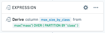
… then the resulting table will look like this:

name	class	mass	max_size_by_class
Jiddat al Harasis 450	H3.7-5	217.741	3879
Ramlat as Sahmah 422	H3.7-5	3879	3879
…
Beni Semguine	H5-an	18	33.9
Miller Range 07273	H5-an	33.9	33.9
…
Allan Hills 88102	Howardite	8.33	40000
Allan Hills 88135	Howardite	4.75	40000
…
Yamato 81020	CO3.0	270.34	3912
Northwest Africa 2918	CO3.0	237	3912

To calculate the cumulative sum (running total) of mass by meteorite class over time:

SUM("mass") OVER (PARTITION BY "class"
    ORDER BY "year" ASC
    ROWS BETWEEN UNBOUNDED PRECEDING AND CURRENT ROW
)

This partitions the table by meteorite class, sorts each partition by date, and then for each row, calculates the sum of the current row plus all previous rows in the mass column, and adds that sum as a new column in the current row.

To calculate the total (not running) sum of mass by meteorite class:

SUM("mass") OVER (PARTITION BY "class")

This aggregation might not be useful by itself, but if we expand it, we can calculate a more interesting statistic – what percentage does this meteorite contribute to the total mass for the class?

"mass" / (SUM("mass") OVER (PARTITION BY "class")) * 100

To calculate the total number (count) of meteorites found for each class:

COUNT("id") OVER (PARTITION BY "class")

Non-determinism

:::callout{theme="warning" title="Warning"} When using ROW_NUMBER, FIRST, LAST, ARRAY_AGG, or ARRAY_AGG_DISTINCT, in a window function, be careful of nondeterminism. Imagine we are partitioning by column A and ordering by column B. If for the same value of column A, there are multiple rows with the same value of column B, the results of these window functions may be non-deterministic -- they may produce different results given the same input data and logic. :::

---

中文翻译

窗口函数(Window functions)

PostgreSQL文档 ↗对窗口函数(Window functions)的定义如下：

窗口函数(Window function)对一组与当前行存在某种关联的表行执行计算。这类似于可以使用聚合函数(Aggregate function)完成的计算类型。但与常规聚合函数不同，使用窗口函数不会导致行被分组为单个输出行——各行保留其独立身份。在幕后，窗口函数能够访问的不仅仅是查询结果的当前行。

本文档解释了一些您可能希望在Contour表达式中使用的窗口函数的语法。有关窗口函数的更多背景信息，请参阅以下其他资源：

• 窗口函数(PostgreSQL文档) ↗
• SQL窗口函数(Mode Analytics教程) ↗
• SQL窗口函数简介(Apache Drill) ↗
• 分析函数(Oracle文档) ↗

基本语法

最基本的窗口函数可以分解为：

<函数> OVER <某个窗口>

其中函数是支持的聚合函数之一，窗口是表中行的子集。

您可以通过使用()来省略窗口——这会将函数应用于表中的所有行。

以下示例将向每一行添加一个条目，其中包含date列中的最大值。

MAX("date") OVER ()

PARTITION BY

您还可以在窗口定义之前添加可选的PARTITION BY子句。PARTITION BY根据给定列中的值对窗口内的行进行分组。然后，聚合函数将分别应用于每个分区。

例如，在一个包含人员记录的表中，以下表达式计算男性和女性的总数，并为每一行添加一个计数，对应其性别值：

COUNT("person_id") OVER (PARTITION BY "gender")

ORDER BY

对于确实定义了窗口的表达式，您必须指定窗口的边界以及如何对表中的行进行排序。这个子表达式可以简化为：

<如何排序表> ROWS BETWEEN <起始位置> AND <结束位置>

其中"如何排序表"包括(1)按哪一列排序以及(2)按升序还是降序排序。

指定窗口边界（"起始位置"和"结束位置"）有以下几种可能：

• UNBOUNDED PRECEDING：从表的开头到当前行。
• n PRECEDING（例如2 PRECEDING）：从当前行之前的n行到当前行。
• CURRENT ROW
• n FOLLOWING（例如5 FOLLOWING）：从当前行到当前行之后的n行。
• UNBOUNDED FOLLOWING：从当前行到表的末尾。

以下是一个示例表，标注了上述每种可能性：

FIRST_NAME |
------------
Adam       |<-- UNBOUNDED PRECEDING
...        |
Alison     |
Amanda     |
Jack       |
Jasmine    |
Jonathan   | <-- 1 PRECEDING
Leonard    | <-- CURRENT ROW
Mary       | <-- 1 FOLLOWING
Tracey     |
...        |
Zoe        | <-- UNBOUNDED FOLLOWING

(来源： blog.jooq.org ↗)

因此，给定一个包含销售记录的表，您可以使用以下表达式来查找最近5次销售的平均销售额：

AVG("sale_value") OVER (ORDER BY "date_of_sale" ASC 
    ROWS BETWEEN 4 PRECEDING AND CURRENT ROW)

"最近5次销售"就是窗口。OVER之后的子表达式按日期对表进行排序，然后对于每一行，计算前4行和当前行的平均值。

综合运用

以下复杂示例综合了上述所有语法。 此表达式显示按产品类别分组、截至当前销售的累计销售数量。

COUNT("sale_id") OVER (PARTITION BY "product_category" 
    ORDER BY "date_of_sale" ASC 
    ROWS BETWEEN UNBOUNDED PRECEDING AND CURRENT ROW)

请注意，条目现在按分区排序——换句话说，首先对表进行分区，然后在每个分区内对行进行排序。

更多示例

假设您有一个记录已购买物品的表。您可以使用以下窗口函数来推导出一个用于计算购买累计总额的新列：

SUM("item_cost") OVER (ORDER BY "purchase_date" ASC 
    RANGE BETWEEN UNBOUNDED PRECEDING AND CURRENT ROW )

要计算按类别分组的累计总额，您可以添加分区：

SUM("item_cost") OVER (PARTITION BY "category" 
    ORDER BY "purchase_date" ASC 
    RANGE BETWEEN UNBOUNDED PRECEDING AND CURRENT ROW)

这将按"category"列对行进行分区，按购买日期对每个类别内的行进行排序，并计算该类别中所有物品成本的累计总额。

陨石数据示例

您可以使用陨石着陆数据集自行尝试以下示例。该数据集来自陨石学会，通过NASA数据门户 ↗获取。

此表达式计算每个类别中最大的陨石：

MAX("mass") OVER (PARTITION BY "class" )

如果我们使用上述窗口函数推导出一个新列max_size_by_class：

…那么结果表将如下所示：

name	class	mass	max_size_by_class
Jiddat al Harasis 450	H3.7-5	217.741	3879
Ramlat as Sahmah 422	H3.7-5	3879	3879
…
Beni Semguine	H5-an	18	33.9
Miller Range 07273	H5-an	33.9	33.9
…
Allan Hills 88102	Howardite	8.33	40000
Allan Hills 88135	Howardite	4.75	40000
…
Yamato 81020	CO3.0	270.34	3912
Northwest Africa 2918	CO3.0	237	3912

要计算按陨石类别随时间变化的累计质量总和（运行总计）：

SUM("mass") OVER (PARTITION BY "class"
    ORDER BY "year" ASC
    ROWS BETWEEN UNBOUNDED PRECEDING AND CURRENT ROW
)

这将按陨石类别对表进行分区，按日期对每个分区进行排序，然后对于每一行，计算当前行加上mass列中所有先前行的总和，并将该总和作为新列添加到当前行。

要计算按陨石类别划分的总（非运行）质量总和：

SUM("mass") OVER (PARTITION BY "class")

这种聚合本身可能不太有用，但如果我们对其进行扩展，可以计算出一个更有趣的统计指标——该陨石占其类别总质量的百分比是多少？

"mass" / (SUM("mass") OVER (PARTITION BY "class")) * 100

要计算每个类别发现的陨石总数（计数）：

COUNT("id") OVER (PARTITION BY "class")

非确定性(Non-determinism)

:::callout{theme="warning" title="警告"} 在窗口函数中使用ROW_NUMBER、FIRST、LAST、ARRAY_AGG或ARRAY_AGG_DISTINCT时，请注意非确定性。假设我们按列A进行分区并按列B进行排序。如果对于列A的相同值，存在多行具有相同的列B值，则这些窗口函数的结果可能是非确定性的——给定相同的输入数据和逻辑，它们可能会产生不同的结果。 :::