Forecast time series（预测时间序列）

You can create forecasts in Quiver using the Time series forecast transform. A forecast is a projection forward in time of an existing time series plot in your analysis. Forecasts in Quiver are built visually and interactively. The result of a forecast is a time series plot representing the forecasted data; this time series plot can be further transformed using Quiver’s time series transforms.

Input type

Time series

Output type

Time series

Usage information

Functionality	Availability
Standard Quiver card	Supported
Transform table transform	Unsupported

Create a forecast

To illustrate this section, we use the linear forecast as an example. Sections below give more details about each type of forecast.

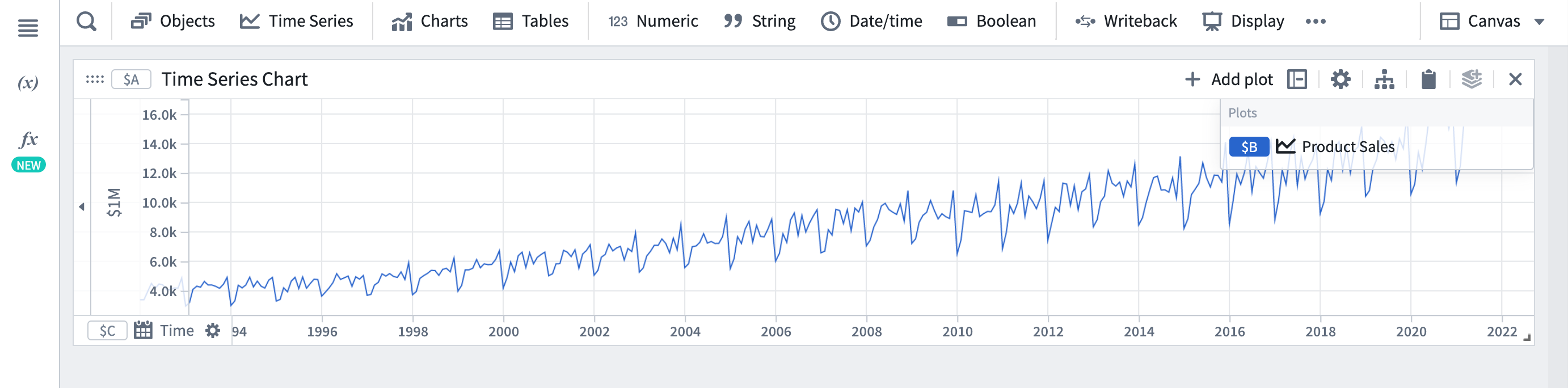
1. Add the time series you would like to forecast to your Quiver analysis by clicking Time Series from the analysis top bar to open the search bar. In our example, we want to forecast the sales of a product.

1. Select Time Series Forecast from the Time Series menu.

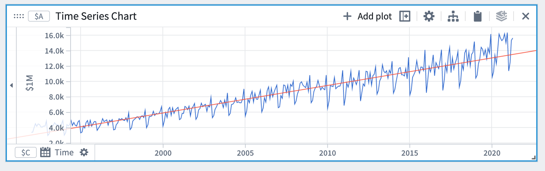
1. In the forecast editor, select the linear forecast type and then select the plot you added at step 1 as the input plot.

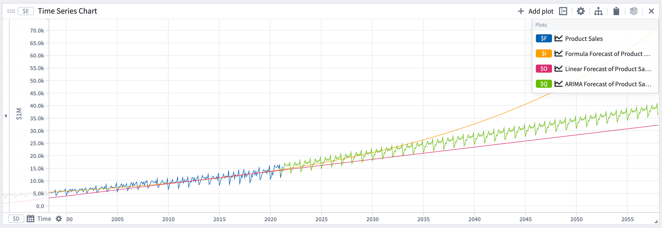
This will produce a time series plot (in this case, a line), that is by default fitted to the entire range of the input plot. Note that the time axis will remain the same as it was for the input time series plot. To see the forecast further into the future, you can zoom out on the x-axis.

You can find the values of the coefficients under the Forecast Details section of the forecast editor.

In the linear forecast example, the coefficients are m (the slope) and c (the offset).

Optional steps

1. To restrict the fitting to a particular time range, turn on the Use Training Time Range toggle and select a time range parameter.

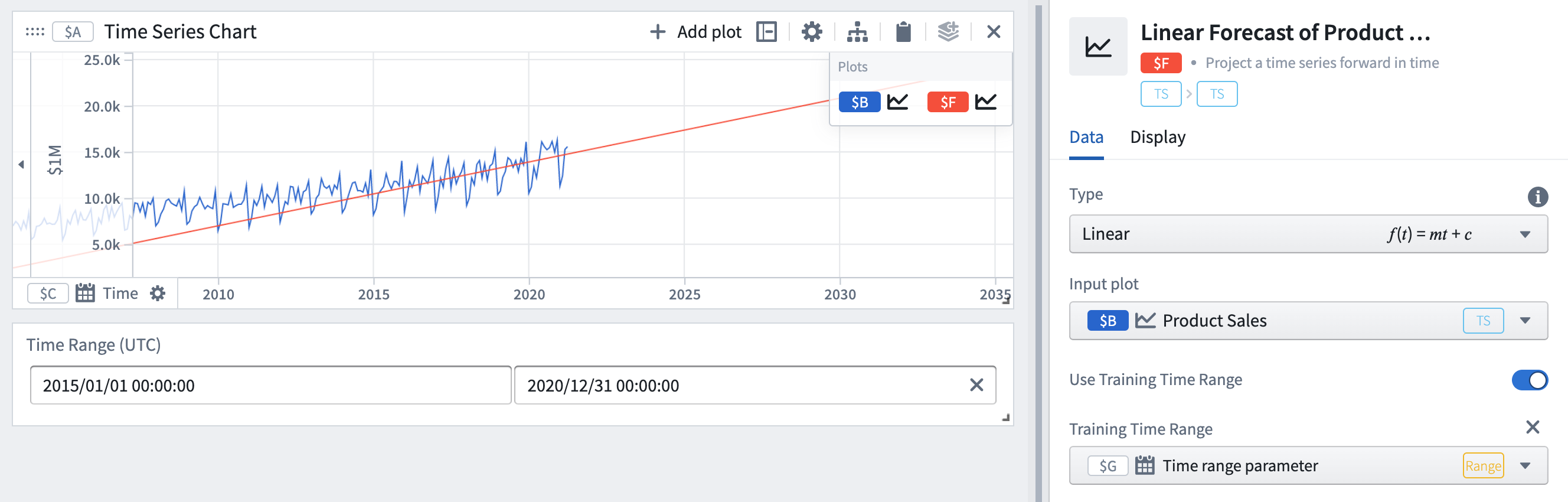
Here we have set the training time range to be 2015-2020 instead of the entire history. As a result, the parameters (slope and offset) of the forecast have changed to make the forecast more accurate for the training time range. This can be useful if you believe certain times will be more indicative of future behavior.

1. Set coefficients boundaries. In the Coefficients section of the editor, switch on the toggles for the coefficients you want to set boundaries on. In this example, setting a boundary on the slope coefficient of this forecast changes both coefficients.

1. Choose a loss definition. The default loss is the sum of squared differences, and the other options are the maximum absolute difference and the sum of absolute differences. When fitting the forecast to the training data, parameters will be selected to minimize the loss. Different types of loss will result in different forecasts. For more details refer to the losses section.

In our example, changing the loss definition results in different forecast coefficients.

The different types of forecasts

In this section, we detail the different types of forecast and their configuration options. For the remainder of the documentation, we refer to the quantity to be forecasted as y or y(t) to denote y at time t.

Constant

The constant forecast assumes the quantity y will remain constant.

Mathematical form: y = a

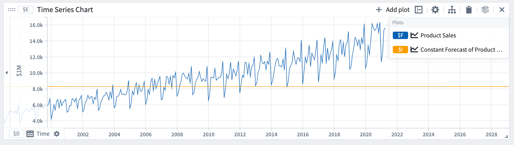
In our example, we can see that the constant forecast does not capture the slope or periodicity in the data.

Linear

The linear forecast assumes the quantity y will follow a linear trend.

Mathematical form: y = a*t + b

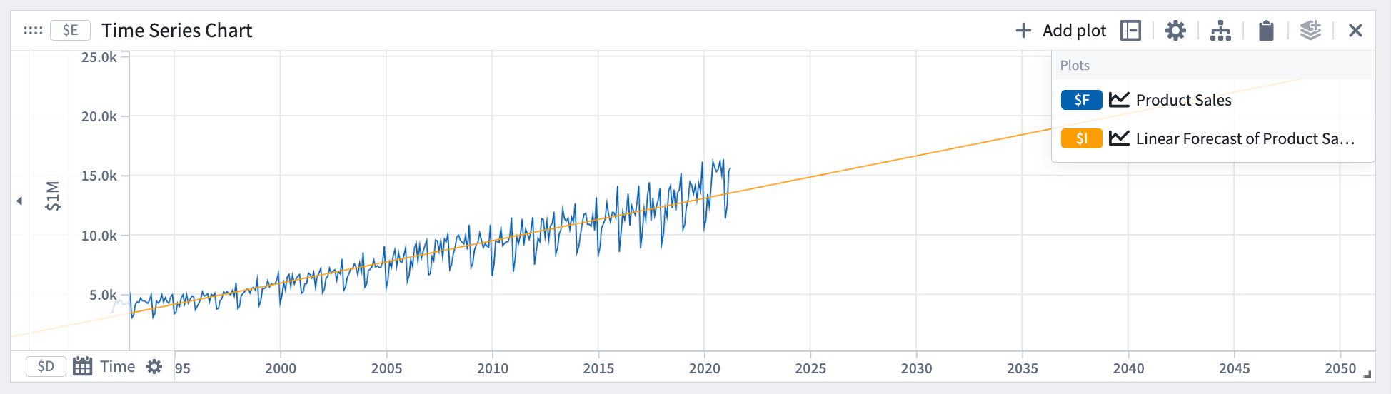
In our example, the linear forecast captures the slope but not the periodicity in the data.

Formula

Formula forecasts can be used when there is periodicity in the data, and the quantity is following some physical process that ebbs and flows. For example, ambient temperature exhibits both daily and yearly periodicity. The formula forecast allows you to fit a sinusoidal curve.

The formula forecast assumes the quantity y follows a governing equation.

Mathematical form: y = f(t)

Examples:

• Exponential formula

• Sinusoidal formula

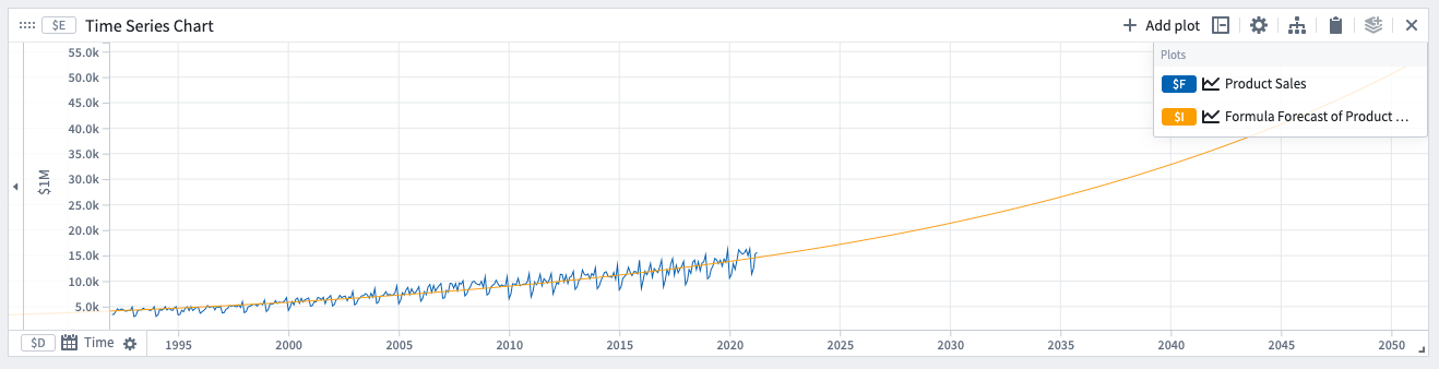
Example forecast with an exponential formula. The coefficients determined by the model are displayed in the expression under Forecast details.

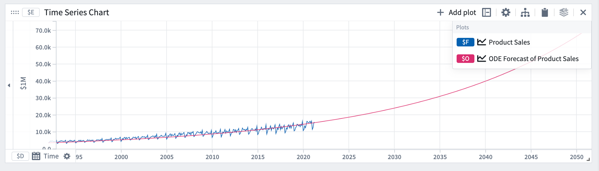
ODE (Ordinary differential equation)

ODE can be used to forecast a quantity that is governed by an Ordinary Differential Equation. The ODE forecast assumes the derivative (rate of change) of the quantity y follows a governing equation.

Mathematical form:

• 1st order

• 2nd order

Examples:

• Exponential growth (λ>0) or decay (λ<0)

• Newton's 2nd law (F=m*a)

• Spring mass system, simple harmonic oscillator

To define your ODE forecast, add the governing equation to the expression box with the unknowns defined as coefficients using the @ prefix and a letter. For example, for exponential growth we have @k * y, where y is the quantity.

In this example, we used an ODE forecast using the exponential growth equation.

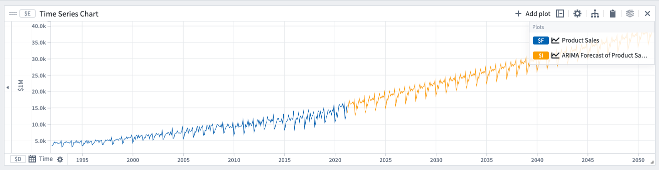
ARIMA (Autoregressive integrated moving average)

This forecast is indicated when there is periodicity in the data coming from some pattern of life. For example, retail sales exhibit some weekly periodicity if people are more likely to shop on certain days of the week.

Mathematical form (non-seasonal):

Where: yd​ is y after differences (subtract consecutive values) have been taken d times.

Options

Auto

Selecting the auto option will set the following ARIMA parameters for you automatically. If you prefer, you can change the parameters manually until you get a satisfactory fit. If selecting the ARIMA parameters manually, bias toward smaller numbers as a simpler model with less terms will generalize better.

ARIMA parameters:

• Number of autoregressive terms (p).
• Number of differences taken (d).
• Number of moving average terms (q).

Seasonal

It is possible to add a seasonal component to the model. To do so, switch the seasonal toggle and specify the period of seasonality. For example, if you have daily data with weekly periodicity, enter 7.

If the auto option is off, the following parameters will appear:

• Number of seasonal autoregressive terms (P).
• Number of seasonal differences taken (D).
• Number of seasonal moving average terms (Q).

The different types of losses

For certain forecast types, you can choose the loss definition used when fitting the forecast. When fitting the forecast to the training data, the coefficients will be selected to minimize the loss. Different types of loss will result in different forecasts.

Sum of squared differences (default)

The square root of the sum of square differences between the target series points y[i] ​and the forecast f[i] ​points within the training time range. Equivalent to the L2​ norm of the error.

Sum of absolute differences

The sum of absolute differences between the target series points ​and the forecast points within the training time range. Equivalent to the L1​ norm of the error.

Maximum absolute difference

The maximum absolute difference between the target series points and the forecast points within the training time range. Equivalent to the L-infinity (L∞​) norm of the error.

---

中文翻译

预测时间序列

您可以使用时间序列预测转换在 Quiver 中创建预测。预测是对分析中现有时间序列图在时间上的向前投影。Quiver 中的预测以可视化和交互方式构建。预测的结果是一个表示预测数据的时间序列图；该时间序列图可以使用 Quiver 的时间序列转换进行进一步处理。

输入类型

时间序列

输出类型

时间序列

使用信息

功能	可用性
标准 Quiver 卡片	支持
转换表转换	不支持

创建预测

为了说明本节内容，我们以线性预测为例。下文各节将详细介绍每种预测类型。

1. 通过点击分析顶部栏的时间序列打开搜索栏，将您想要预测的时间序列添加到 Quiver 分析中。在我们的示例中，我们想要预测某产品的销售额。

1. 从时间序列菜单中选择时间序列预测。

1. 在预测编辑器中，选择线性预测类型，然后选择您在步骤 1 中添加的图作为输入图。

这将生成一个时间序列图（本例中为一条线），默认情况下该图拟合到输入图的整个范围。请注意，时间轴将与输入时间序列图保持一致。要查看更远的未来预测，您可以缩小 x 轴。

您可以在预测编辑器的预测详情部分找到系数的值。

在线性预测示例中，系数为 m（斜率）和 c（截距）。

可选步骤

1. 要将拟合限制在特定时间范围内，请打开使用训练时间范围开关并选择时间范围参数。

这里我们将训练时间范围设置为 2015-2020 年，而不是整个历史数据。因此，预测的参数（斜率和截距）发生了变化，使得预测在训练时间范围内更加准确。如果您认为某些时间更能指示未来行为，这将非常有用。

1. 设置系数边界。在编辑器的系数部分，为您想要设置边界的系数打开开关。在此示例中，为此预测的斜率系数设置边界会改变两个系数。

1. 选择损失定义。默认损失是平方差之和，其他选项是最大绝对差和绝对差之和。在将预测拟合到训练数据时，将选择参数以最小化损失。不同类型的损失会导致不同的预测。更多详情请参考损失部分。

在我们的示例中，更改损失定义会导致不同的预测系数。

不同类型的预测

在本节中，我们将详细介绍不同类型的预测及其配置选项。在本文档的其余部分，我们将要预测的量称为 y 或 y(t)，表示时间 t 处的 y。

常数

常数预测假设量 y 将保持不变。

数学形式：y = a

在我们的示例中，可以看到常数预测未能捕捉到数据中的斜率或周期性。

线性

线性预测假设量 y 将遵循线性趋势。

数学形式：y = a*t + b

在我们的示例中，线性预测捕捉到了斜率，但未能捕捉到数据中的周期性。

公式

当数据中存在周期性，且该量遵循某种具有涨落规律的物理过程时，可以使用公式预测。例如，环境温度表现出日周期性和年周期性。公式预测允许您拟合正弦曲线。

公式预测假设量 y 遵循一个控制方程。

数学形式：y = f(t)

示例：

• 指数公式

• 正弦公式

使用指数公式的预测示例。模型确定的系数显示在预测详情下的表达式中。

ODE（常微分方程）

ODE 可用于预测由常微分方程控制的量。ODE 预测假设量 y 的导数（变化率）遵循一个控制方程。

数学形式：

• 一阶

• 二阶

示例：

• 指数增长（λ>0）或衰减（λ<0）

• 牛顿第二定律（F=m*a）

• 弹簧质量系统，简谐振子

要定义您的 ODE 预测，请将控制方程添加到表达式框中，未知数使用 @ 前缀加字母定义为系数。例如，对于指数增长，我们有 @k * y，其中 y 是量。

在此示例中，我们使用了指数增长方程的 ODE 预测。

ARIMA（自回归积分滑动平均）

当数据中存在来自某种生活模式的周期性时，适合使用此预测。例如，如果人们更倾向于在一周中的某些天购物，零售额会表现出周周期性。

数学形式（非季节性）：

其中： yd 是 y 经过 d 次差分（减去连续值）后的结果。

选项

自动

选择自动选项将自动为您设置以下 ARIMA 参数。如果您愿意，可以手动更改参数，直到获得满意的拟合效果。如果手动选择 ARIMA 参数，请倾向于较小的数字，因为项数较少的简单模型泛化效果更好。

ARIMA 参数：

• 自回归项数 (p)。
• 差分次数 (d)。
• 滑动平均项数 (q)。

季节性

可以为模型添加季节性成分。为此，请打开季节性开关并指定季节性周期。例如，如果您有日数据且具有周周期性，请输入 7。

如果自动选项关闭，将出现以下参数：

• 季节性自回归项数 (P)。
• 季节性差分次数 (D)。
• 季节性滑动平均项数 (Q)。

不同类型的损失

对于某些预测类型，您可以选择拟合预测时使用的损失定义。在将预测拟合到训练数据时，将选择系数以最小化损失。不同类型的损失会导致不同的预测。

平方差之和（默认）

训练时间范围内目标序列点 y[i] 与预测点 f[i] 之间平方差之和的平方根。等同于误差的 L2 范数。

绝对差之和

训练时间范围内目标序列点与预测点之间绝对差之和。等同于误差的 L1 范数。

最大绝对差

训练时间范围内目标序列点与预测点之间的最大绝对差。等同于误差的 L-无穷大（L∞）范数。